
Geothermal investment decisions depend on a connection between physical heat delivery, business expenditure, and the conditions under which a project operates. Evidence of lower energy expenditure after adoption is useful, but its meaning depends on whether the reported quantity is a price, an annual bill, or a cost per unit of production. A similar distinction separates a reduction in annual carbon dioxide emissions from a reduction in the carbon intensity of a product. These differences matter particularly when business evidence is available through summary tables: a reader can recover some operating comparisons exactly, while other conclusions require measurements that the tables do not contain.
The diversity of geothermal applications makes this an energy-specific problem. International assessments distinguish direct heat uses across buildings, agriculture, aquaculture, and industrial activities, alongside geothermal electricity generation [1]. Long-run inventories document substantial differences in the distribution and growth of these applications [2]. A business purchasing geothermal heat is not equivalent to an enterprise operating a geothermal power plant. Temperature requirements, delivery arrangements, and the displaced energy service influence what an operating reduction can mean. Pooling such applications without information on their energy boundaries can obscure mechanisms even when the reported average change is numerically precise.
Techno-economic work on deep direct use shows why a reduction in an observed unit energy cost is only one component of investment appraisal. Feasibility depends on resource conditions, infrastructure, thermal demand, and the economic assumptions used to evaluate a project [3]. Research on shallow geothermal industrial applications likewise connects performance to the particular installation and its operating requirements [4]. These studies support careful specification of an energy service; they do not supply missing expenditure or consumption quantities for a different group of firms. The absence of those quantities limits the translation of a business comparison into a payback period or a regional investment recommendation.
Italy also contains resource opportunities with distinct development histories. Assessment of geothermal opportunities in Italian oil and gas fields illustrates the importance of subsurface characteristics and existing infrastructure [5]. The uncertainty attached to exploration is itself a substantive economic issue, because uncertainty in the resource changes the information available when capital is committed [6]. Neither a national resource estimate nor a favorable mean operating comparison determines the return to a particular enterprise. Linking those levels requires information about the adopted technology, the heat requirement, the financing structure, and the alternative energy supply.
Environmental interpretation presents an analogous difficulty. Life-cycle work on Italian geothermal power plants explicitly examines atmospheric emissions and the choices made in evaluating them [7]. A complete inventory-based assessment requires more than a single annual carbon dioxide total [8]. Studies of enhanced geothermal heat in the Upper Rhine region demonstrate the relevance of construction, operation, and the delivered heat service to a climate assessment [9]. Such findings explain why technology and accounting boundaries matter; their numerical emission factors cannot simply be assigned to unidentified Italian business installations. A measured corporate reduction and a life-cycle advantage answer different questions.
Social acceptance is equally resistant to interpretation through a single variable. A systematic review identifies acceptance as a multidimensional issue involving technological characteristics, institutions, perceptions, and local circumstances [10]. Deliberative engagement in central Italy examines how participants discuss and assess geothermal development [11]. Public engagement in southern Italy provides further evidence that local concerns cannot be reduced to the physical availability of a resource [12]. These studies make risk communication relevant, but they do not imply that every observed association between communication and opposition is the effect of communication itself.
A firm may communicate because it has a mature project, experienced staff, established institutional relationships, or prior contact with residents. Opposition may also alter the timing and content of subsequent communication. The binary observation that communication occurred therefore lacks a complete temporal account of how an interaction developed. Work on affective responses to deep geothermal energy shows that perceptions of induced seismicity belong within that account [13]. Evidence from political and social contestation in Alsace further illustrates that acceptance depends on project context [14]. A strong contingency-table association can coexist with uncertainty about these underlying processes.
The analytical challenge is to separate three questions that are often treated together: what the available quantities identify, how uncertainty should be expressed, and what causal interpretation the design permits. Ecologic and aggregate evidence can support legitimate analyses, but it does not generally determine individual relationships merely because its summaries are internally precise [15]. Likewise, a small probability under a null model does not measure the magnitude, practical value, or causal meaning of a finding [16]. A useful business interpretation must therefore retain both the units of the outcome and the limitations of its observation process.
Means and standard deviations nevertheless preserve substantial information. The standard deviation of a paired difference, together with the marginal standard deviations, determines the covariance between periods. A contingency table determines an exact association probability and supports interval estimates even when one group reports no events. A fitted least-squares line with an intercept must pass through its sample means. These identities allow substantive claims to be checked without simulating firms or pretending that aggregate information provides individual trajectories. Their value lies in identifying both what can be recovered and where additional evidence becomes necessary.
The present research asks: Which conclusions about geothermal-related business changes remain identifiable from the Italian firm summaries when zero-event uncertainty, outcome classification, paired dependence, common time changes, and regression compatibility are considered explicitly? The question concerns the information supporting a decision, rather than another estimate of how much geothermal adoption lowers costs or emissions. The contribution is an integrated calculation of these distinct evidential limits for the same 40-firm record. Exact binary intervals, finite outcome reassignment, covariance recovery, translated intervals under common time shifts, and rounding-aware regression checks produce quantities that are absent from the descriptive averages alone.
This approach follows an estimation-oriented interpretation in which the size and uncertainty of a contrast receive direct attention [17]. It also maintains a boundary between calculated sensitivity and observed behavior. Reassigning an outcome label is a numerical perturbation, not evidence that the label was wrong; subtracting a common time shift is an assumption, not an estimated control-group trend. The resulting conclusions concern the documented sample and the specified assumptions. They provide an auditable account of where the available evidence is strong, where it is conditional, and where an investment or environmental claim cannot be obtained from the reported quantities.
The numerical evidence consists of 40-firm Italian investigation [18]. The analytical collection accompanying this manuscript contains transcribed summary quantities, derived covariances, exact probability calculations, and explicitly defined numerical perturbations. Recruitment was purposive and covered Tuscany, Piedmont, Campania, and Sicily, with applications including aquaculture and wine production. Forty of 65 selected enterprises participated, equivalent to 61.54%. Respondents occupied managerial or technical positions connected with energy decisions. The operating quantities compare averages over the three years preceding adoption with averages over the three years following adoption. Consequently, the paired sample size is 40, not 240 firm-years. Dates of adoption, annual trajectories, recruitment strata, and the characteristics of the 25 nonparticipants are unavailable. Geographic names identify the recruitment setting; they do not establish regional sample sizes or regional representativeness.
The before and after windows also require careful treatment of the time unit. Averaging three annual observations within a firm does not establish that the annual observations were independent, equally complete, or exposed to the same price conditions. The reported difference is a contrast between two period averages. Multiplying that contrast by three would describe a different quantity and would require confirmation of how annual costs and emissions were aggregated. The calculation therefore retains the period-average interpretation throughout. Firm-level pairing is preserved conceptually even though the individual values are unavailable for inspection.
The prose variable definition describes energy cost as an annual total, whereas the numerical comparisons assign euros per megawatt-hour. Energy expenditure is therefore interpreted conditionally as a unit cost, following those numerical comparisons; the underlying accounting definition remains unresolved. Annual carbon dioxide emissions are expressed in tonnes. The former quantity is a unit cost, whereas the latter is an annual total averaged within each period. They must not be combined as if both were annual expenditures or both were intensities. No energy-consumption weights, output quantities, capital expenditures, financing terms, or life-cycle emission inventories are available. Accordingly, total monetary savings, payback periods, and emissions per unit of product cannot be calculated.
Let \(C=1\) denote that a firm communicated geothermal risks, and let \(Y=1\) denote reported criticism or resistance. The labeled table contains \((Y=1,Y=0)=(0,27)\) for communicating firms and \((11,2)\) for noncommunicating firms. Pearson’s and likelihood-ratio independence statistics, Fisher’s two-sided exact test, Cramér’s \(V\), and the signed binary association coefficients are retained as descriptive calculations. Test selection in a small contingency table requires an explicit convention [19]. The exact test sums fixed-margin hypergeometric probabilities no greater than the probability of the observed table. It is a conditional test of association, with no adjustment for firm size, location, project maturity, or the timing of communication.
The principal binary contrast is the observed risk difference,
Its uncertainty is described with the Newcombe interval constructed from separate Wilson score intervals [20], [21]. This avoids treating a zero observed event proportion as having zero uncertainty, a boundary problem for simple normal intervals [22]. A separate exact binomial interval describes the communicating group [23]. For zero events among \(m\) firms, the upper one-sided 95% bound satisfies
The two-sided 95% exact interval instead uses 0.025 in the upper-tail calculation. These bounds are different inferential statements and are labeled separately. They assume a binomial observation model; purposive recruitment and possible dependence among neighboring projects limit their population interpretation. The two group intervals and the difference interval should not be assessed by checking whether their endpoints overlap. The difference interval combines the component score limits according to its own construction. If the group estimates are \(p_1\) and \(p_0\), with score limits \((l_1,u_1)\) and \((l_0,u_0)\), its lower endpoint subtracts \(\sqrt{(p_1-l_1)^2+(u_0-p_0)^2}\) from \(p_1-p_0\), and its upper endpoint adds \(\sqrt{(u_1-p_1)^2+(p_0-l_0)^2}\). This explicit calculation preserves the asymmetry introduced by the zero event count and avoids substituting a symmetric interval around an estimated probability of zero.
Outcome-label sensitivity adapts the idea of counting changes required to cross a test threshold [24]. Complete enumeration keeps the communication group sizes fixed. Let \(a\) and \(c\) be the opposition counts in the communicating and noncommunicating groups after reassignment. For \(0\leq a\leq27\) and \(0\leq c\leq13\), the perturbed table is
For each maximum number of changes \(k\), all allocations requiring at most \(k\) individual label changes are evaluated. The threshold is the smallest \(k\) for which at least one allocation produces a two-sided Fisher probability of at least 0.05. This is a deliberately adverse reassignment calculation, not an estimate of the actual misclassification rate. Communication labels, nonparticipation, and unmeasured determinants of both variables are held outside this calculation and remain separate limitations.
For each outcome, let \(B_i\) and \(A_i\) be the before and after period averages, and define \(D_i=B_i-A_i\). Positive \(D_i\) denotes a reduction. The mean paired contrast and its two-sided Student interval are
The paired \(t\) statistic uses the same denominator. The interpretation follows the distinction between statistical uncertainty and other sources of error [25]. The interval is model-based, conditional on the summary quantities, independent firm-level differences, and a sufficiently adequate normal approximation for their mean. Exact Student calibration requires normally distributed differences; the summaries cannot establish this condition or exclude influential observations. It is not a probability statement about a fixed parameter after observation, nor a range containing 95% of individual firm changes. The standard error is computed from the difference standard deviation, never by treating the two periods as independent samples.
The covariance and correlation between periods are identified algebraically:
This calculation requires the same paired firms and sample-variance convention in all three quantities. A feasible correlation establishes compatibility of the variances; it does not verify the underlying measurements. To show the consequence of retaining the paired structure, the counterfactual independent-sample standard error is calculated as \(\sqrt{(s_B^2+s_A^2)/40}\). It is used solely as an information-loss diagnostic, not as a second test of the same hypothesis.
The lower endpoint is additionally evaluated as a function of an assumed correlation, \(L(r)=\bar D-t_{0.975,39}\sqrt{(s_B^2+s_A^2-2rs_Bs_A)/40}\). The range \(-1\leq r\leq1\) defines an unrestricted second-moment envelope, not uncertainty in the recovered correlation or alternate pairings compatible with every feature of the firms. Nonnegative outcome support can restrict attainable correlations further. A positive lower endpoint throughout this larger envelope also remains positive over any admissible subset.
Two standardizations answer different questions because repeated-measures and marginal standardizers capture different variation [26], [27]. The paired standardized change is \(d_z=\bar D/s_D\). A second quantity divides the mean change by the root mean square of the two marginal standard deviations, \(d_{\mathrm{RMS}}=\bar D/\sqrt{(s_B^2+s_A^2)/2}\). The first reflects variation in changes; the second reflects dispersion in outcome levels. Neither is a standardized causal effect. Relative reduction is separately expressed as \(100\bar D/\bar B\), a ratio of sample means that must not be substituted for the unobserved mean of firm-specific percentage reductions.
A Wilcoxon signed-rank comparison belongs to the documented analytical procedure, but its signed ranks cannot be recovered from means and variances. No rank statistic or probability is generated here. The same restriction applies to claims that every individual difference is positive. Reporting an unavailable rank calculation as confirmation would create evidence absent from the numerical record.
Suppose an average reduction \(\delta\) would have occurred over the same periods without the change in geothermal use. This quantity can represent a common price movement for unit costs or a change in operating activity for emissions, expressed in the corresponding outcome units. It is not estimated from the available tables. A common deterministic shift is subtracted from every firm’s difference, leaving the difference standard deviation unchanged. A conditional attribution calculation is
If only \(0\leq\delta\leq B\) is imposed, the sensitivity range for the adjusted point estimate is \([\bar D-B,\bar D]\), and the union of the translated intervals is \([L_D-B,U_D]\). Positivity of the lower endpoint is retained only while \(B<L_D\). This bound describes the strength of an assumption required to maintain a positive comparison; it does not show that the assumption holds.
The shifts make assumptions about systematic change explicit, consistent with quantitative bias analysis [28]. The shifts are deterministic sensitivity inputs. They are neither measured confounders nor random draws from a fitted distribution. Their interpretation is therefore narrower than a fully adjusted causal analysis. Subtracting a common mean shift cannot address selective adoption, different counterfactual trends across firms, endogenous production changes, or disagreement about which emissions belong within a firm’s accounting boundary. Those mechanisms require additional design information.
Mathematical constraints have been used to check the compatibility of reported summaries [29]. The integer-granularity requirement of that work is not imposed on the continuous quantities here. Recalculation of test quantities likewise checks internal reporting without establishing the authenticity of observations [30]. For an ordinary least-squares regression with an intercept, fitted to the same cases and outcome definition, the fitted line passes through the sample means:
This identity is checked for the geothermal-share regressions using both before-minus-after and after-minus-before conventions. A favorable interpretation must satisfy the identity before a slope can support a quantitative claim about increasing geothermal use. The mean identity follows directly from the least-squares intercept condition: residuals sum to zero, so their mean is zero and the mean fitted value equals the mean observed outcome. It holds regardless of residual normality and does not require a small slope probability. Consequently, this is a compatibility requirement on reported quantities rather than another hypothesis test. Failure cannot be repaired by increasing the sample size stated alongside the regression or by citing its coefficient of determination. Different case selection or transformed variables could change the applicable means, but such changes would need to be documented before a common interpretation was justified. The implied mean share is \((\bar y-\widehat\alpha)/\widehat\beta\). Agreement with a standard deviation or a coefficient of determination cannot substitute for agreement with the mean identity.
Rounding is handled as an interval calculation. A quantity printed to three decimal places represents the displayed value plus or minus 0.0005 under ordinary nearest rounding. All endpoint combinations of the intercept, slope, and mean-share intervals are evaluated to bound the fitted mean. The emissions mean difference receives its printed three-decimal precision interval. For costs, the target interval is derived from the two three-decimal period means, giving a difference uncertainty of 0.001; the less precise printed difference of 8.8 alone is insufficient for this check. Disjoint intervals show that ordinary rounding alone cannot reconcile the quantities under the same-case, same-variable assumptions. They do not identify which entry, sample definition, or transformation is responsible.
The residual standard error and slope uncertainty provide supplementary checks on the predictor dispersion. These calculations retain the linear-model method while restricting its interpretation to quantities supported by mutually compatible summaries. Reported residual normality, serial-correlation, and heteroskedasticity diagnostics cannot be independently recalculated from these regression summaries. No new adoption-response curve is fitted, and the four expert-defined ranges are not assigned artificial midpoints for a regression. Every input and derived value is stored in machine-readable form, with a deterministic Python calculation and separate plotting script supplied in the project archive.
The communication groups contain 27 and 13 firms, respectively, with 11 reported opposition events in total. Thus, 67.50% communicated risks and 27.50% reported opposition under the labeled-table convention. The binary means of 0.325 and 0.725 in Table 1 are complements of these proportions. They could describe reverse-coded indicators, but they must not be interpreted as the proportions of communication and opposition under the present definitions. The visible group labels and integer counts, displayed in Figure 1, provide the unambiguous basis for the present calculation.
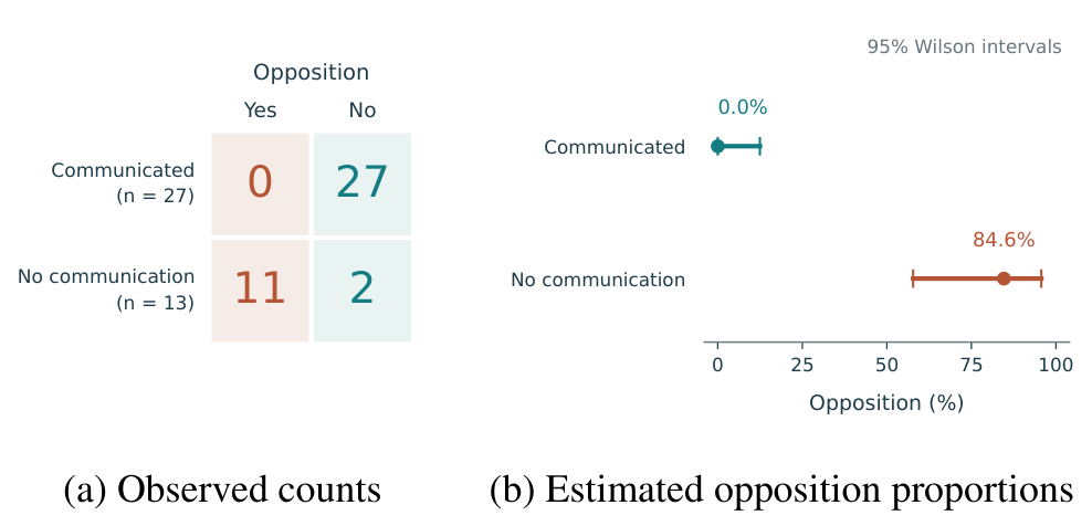
The observed opposition proportions are 0% and 84.62%. Their difference is \(-84.62\) percentage points, with a Newcombe 95% interval from \(-95.67\) to \(-55.02\) percentage points. The magnitude of this contrast is substantial within the responding sample. Pearson’s statistic is 31.5119, the likelihood-ratio statistic is 35.8911, and the two-sided Fisher probability is \(3.374\times10^{-8}\). Cramér’s \(V\) is 0.8876, which is nonnegative by definition; the signed association under the stated coding is \(-0.8876\). For these binary observations, Kendall’s tau-b and Spearman’s rank correlation equal that signed value, while Goodman–Kruskal’s gamma is \(-1\) because tied pairs are excluded. These distinct quantities describe the strength and direction of association without treating a rounded probability of 0.000 as an exact zero.
The absence of opposition in the communicating group does not identify a zero event probability. Eq. (2) gives a one-sided 95% upper bound of 10.50%; the upper endpoint of the two-sided 95% Clopper–Pearson interval is 12.77%. The score intervals displayed in Figure 1 differ slightly because they use another interval construction. Their role is to show the uncertainty associated with the two observed proportions, not to offer competing claims about the number of observed events. No continuity correction or invented event has been added to the contingency table. The observed risk ratio and odds ratio both equal zero when the communicating group is placed in the numerator. That arithmetic does not make their logarithms finite, and it does not make the associated uncertainty disappear. The risk-difference presentation is therefore especially useful for this table: it retains the observed zero, gives the contrast in percentage points, and supplies an interval whose construction remains defined. The exact upper bound answers a complementary question about the communicating group’s event probability. These presentations use the same counts while making distinct statistical statements about them.
These calculations separate two conclusions. The observed groups differ sharply, and an exact conditional independence test regards the labeled table as highly unusual under its null model. At the same time, the 27 communicating respondents do not provide evidence of guaranteed acceptance in another project or period. A risk bound remains informative precisely because the observed count is zero. Neither interval construction accounts for nonparticipation, incomplete reporting of criticism, or common institutional conditions among firms.
Complete enumeration produces 392 distinct tables from Eq. (3). No admissible allocation of eight or fewer outcome-label changes raises the Fisher probability to 0.05. The largest probability attainable with eight changes is approximately 0.03783. Nine changes are sufficient, with five different allocations crossing the threshold. Figure 2 displays the entire finite calculation, preserving the distinction between changes made within each communication group.
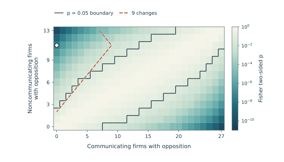
The five minimum-change tables contain respectively \((0,2)\), \((1,3)\), \((2,4)\), \((3,5)\), and \((4,6)\) opposition events in the communicating and noncommunicating groups. Their Fisher probabilities range from 0.05196 to 0.10000. Although each crosses the conventional threshold, each retains a lower observed opposition proportion among communicating firms. Crossing 0.05 therefore does not mean that the contrast has become zero or reversed. At least 11 changes are needed to make the observed risk difference nonnegative under the permitted reassignments.
The required count also depends on which records may change. Restricting changes to communicating firms requires 14 outcome changes; restricting them to noncommunicating firms requires nine. Preserving the total number of opposition events requires ten individual changes because events must be exchanged across groups. The difference is substantive: uncertainty concentrated in one group has a different consequence from uncertainty distributed across both. A single count of nine should consequently be read with its allocation rule, rather than as an intrinsic quality score for the study. The enumeration further clarifies why an outcome error rate cannot be inferred by dividing nine by forty. That quotient would merely express the smallest successful reassignment budget as a share of respondents. It would say nothing about the probability that errors occurred, whether errors were independent, or whether records in both groups were equally likely to be affected. Verification against a second account of each firm’s experience would be needed to estimate classification accuracy. In its absence, the finite calculation describes how the conclusion responds to a declared perturbation and leaves the probability of that perturbation unspecified. This interpretation follows the distinction between significance fragility and the wider stability of a quantitative result [31].
The mean unit energy cost falls from 108.125 to 99.325 euros per megawatt-hour, while mean annual carbon dioxide emissions fall from 346.950 to 303.075 tonnes. The paired reductions and associated uncertainty are summarized in Table 1. The relative changes are 8.14% and 12.65% when expressed as ratios of the mean differences to the respective before-period means. These percentages refer to the aggregate means; the unreported mean of individual percentage changes could differ.
| Quantity | Unit energy cost | Annual CO\(_2\) emissions |
| (EUR/MWh) | (tonnes) | |
| Before-period mean | 108.125 | 346.950 |
| After-period mean | 99.325 | 303.075 |
| Mean reduction | 8.800 | 43.875 |
| Standard deviation of reductions | 3.994869 | 50.588430 |
| Standard error | 0.631644 | 7.998733 |
| Two-sided 95% interval | [7.522,10.078] | [27.696,60.054] |
| Paired \(t\), 39 degrees of freedom | 13.9319 | 5.4852 |
| Reconstructed period correlation | 0.988721 | 0.999817 |
| Paired standardized change, \(d_z\) | 2.2028 | 0.8673 |
| Reduction relative to before mean (%) | 8.1387 | 12.6459 |
The two-sided probabilities are approximately \(1.000\times10^{-16}\) for unit energy cost and \(2.684\times10^{-6}\) for emissions. These values support a positive mean difference within the paired statistical model. They do not establish that the upper interval endpoint is the maximum possible saving, that every firm improved, or that adoption caused the change. In particular, the interval endpoints in Table 1 are two-sided 95% endpoints; labeling them as one-sided 95% limits would assign them a different coverage interpretation.
Dependence between the periods explains much of the precision. Recovered correlations are 0.988721 for unit costs and 0.999817 for emissions. Removing the paired dependence while holding marginal variances fixed would increase the standard error by factors of approximately 4.54 and 12.84. For emissions, large differences in levels across firms coexist with a nearly linear relationship between firms’ before- and after-period levels. Persistent differences in activity scale are compatible with this pattern, but the summaries do not identify the reason for it. For interpretation, the important contrast is between the stability of levels and the spread of changes. A firm with a relatively high emissions level in both periods can contribute strongly to marginal dispersion while contributing a modest difference. Pairing removes that persistent level component from the uncertainty of the average difference. The recovered correlation quantifies the aggregate relationship required for this cancellation. It does not identify which firms contributed most to the mean decline or whether a small group experienced particularly large reductions. Those questions depend on the joint distribution rather than its second moments alone. An unusually high recovered correlation is an implication to verify against records, not an independent validation of those records.
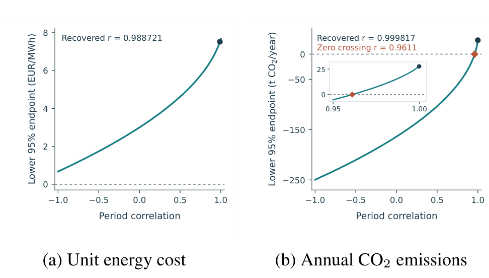
The effect of retaining or discarding that dependence is shown in Figure 3. Holding the marginal variances and mean change fixed, the lower endpoint of the emissions interval becomes positive only when the assumed correlation exceeds approximately 0.9611. In contrast, the unit-cost lower endpoint remains positive throughout the full algebraic range from \(-1\) to \(1\) under the same Student convention. At a correlation of \(-1\), its lower endpoint is approximately 0.674 euros per megawatt-hour. This is a comparison of variance assumptions, rather than a claim that every correlation in that range is compatible with all unreported features of the firms.
Standardization confirms that two apparently different descriptions can both be correct. The paired standardized emissions change is 0.8673, but its value relative to the root mean square of the marginal standard deviations is approximately 0.0955. The corresponding cost quantities are 2.2028 and approximately 0.6862. The denominator determines whether the comparison emphasizes variation in changes or variation in levels. Neither choice is evidence that one physical technology performs better than another, because the sample does not provide technology-specific groups or a common functional unit.
The translated intervals in Figure 4 show how the positive operating comparisons depend on an unmeasured common reduction. For unit energy cost, the lower 95% endpoint reaches zero at 7.522 euros per megawatt-hour; the adjusted point contrast reaches zero at 8.800. For annual emissions, the corresponding quantities are 27.696 and 43.875 tonnes. The difference between each pair distinguishes removal of interval positivity from complete removal of the observed mean reduction.
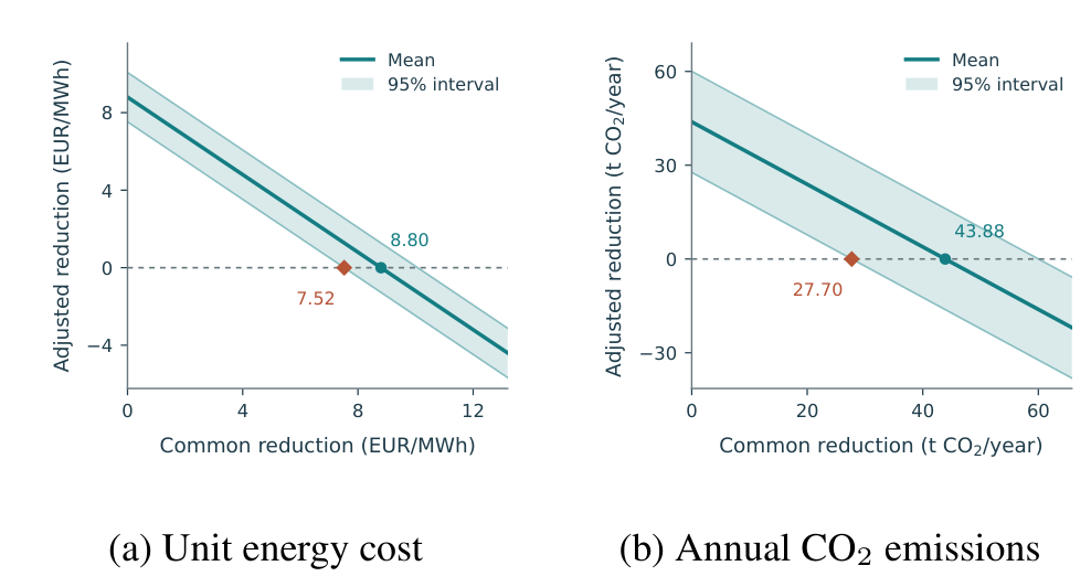
The shifts that remove a positive lower endpoint equal 6.96% of the before-period unit cost and 7.98% of the before-period emissions mean. These percentages describe assumption thresholds, not estimates of actual price declines or output changes. If an analyst could justify a common cost reduction smaller than 7.522 euros per megawatt-hour, the translated lower endpoint would remain positive under Eq. (6). The tables themselves do not provide the evidence needed to justify that restriction. A narrow paired interval therefore does not eliminate uncertainty about what happened during the comparison periods. These thresholds retain their separate outcome units and cannot be combined without additional accounting information and explicit decision preferences.
The printed emissions line is \(\widehat y=104.383-184.196x\), and the printed cost line is \(\widehat y=-0.773-24.435x\). At the mean share of 0.326, their fitted means are 44.335104 tonnes and \(-8.738810\) euros per megawatt-hour. The closest sign conventions are a positive emissions reduction of 43.875 tonnes and a negative cost change of \(-8.800\) euros per megawatt-hour. Even under those favorable conventions, the fitted means do not equal the corresponding paired means, as Table 2 shows.
| Quantity | Emissions line | Cost line |
| Printed intercept | 104.383 | \(-0.773\) |
| Printed share coefficient | \(-184.196\) | \(-24.435\) |
| Fitted mean at \(\bar x=0.326\) | 44.335104 | \(-8.738810\) |
| Closest signed paired mean | 43.875 | \(-8.800\) |
| Required mean share | 0.3284979 | 0.3285042 |
| Rounded fitted-mean lower limit | 44.242343 | \(-8.751691\) |
| Rounded fitted-mean upper limit | 44.427865 | \(-8.725930\) |
| Minimum interval separation | 0.366843 | 0.047309 |
Accounting for displayed precision does not close the differences. The emissions fitted-mean range is 44.242343–44.427865 tonnes, disjoint from the paired-difference range 43.8745–43.8755. The cost fitted-mean range is \(-8.751691\) to \(-8.725930\), disjoint from the \(-8.801\) to \(-8.799\) range obtained by differencing the two three-decimal period means. Figure 5 displays these separate ranges. Using the printed cost difference of 8.8 alone would allow wider rounding uncertainty; the more precise period means are therefore essential to the cost compatibility conclusion.
The intervals in this display have a different meaning from the confidence intervals used for operating reductions. They contain the numerical values compatible with displayed decimal precision under an explicit rounding rule. They do not describe sampling uncertainty, have no confidence level, and cannot be widened by choosing another probability threshold. The observed separation is modest in the physical units, especially for costs, but the mean identity is an exact property of a fitted least-squares line with an intercept. Its relevance is therefore to the consistency of the reported quantities. It does not quantify the practical size of an investment error. The similar implied shares across the two regressions help localize the question that additional records would need to resolve, while leaving the appropriate numerical correction undetermined.
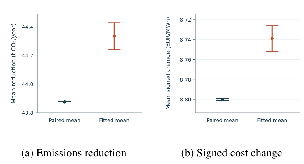
Both fitted lines require a mean geothermal share close to 0.3285, outside the rounding interval 0.3255–0.3265. Their agreement on this implied value suggests a common reporting or definition issue, but does not establish its cause. A transcription error, different analysis cases, or an undocumented variable transformation remains possible. The present calculation identifies incompatibility under stated assumptions, rather than selecting a replacement value for the mean share.
There is a further sign issue. When emissions are expressed as before minus after, a negative share coefficient means that larger shares are associated with smaller positive reductions. When costs are converted to the same reduction convention, their line becomes \(\widehat D=0.773+24.435x\), giving the opposite slope direction. Interpreting both printed negative slopes as larger benefits would therefore combine incompatible definitions of change. These arithmetic and definitional restrictions prevent the coefficients from supporting a common quantitative expansion claim, independently of their reported statistical precision.
The central finding is an asymmetry in the information supporting the two operating outcomes. The mean cost reduction is sufficiently large relative to the marginal dispersions that its positive lower Student endpoint survives the entire variance-only dependence envelope. The emissions comparison obtains its precision from exceptionally strong paired dependence. This difference does not make the emissions reduction unimportant. It means that preserving the link between each firm’s before and after values is especially consequential for that outcome. A report containing only the two emissions means and marginal standard deviations would support a materially weaker account of the comparison.
The recovered covariance should also change how the large spread in emissions is discussed. A standard deviation greater than the mean does not invalidate a paired comparison by itself, because the relevant variability is the variability of the differences. However, a near-perfect recovered correlation does not resolve skewness in those differences. Their distribution, influential firms, and the sensitivity of the mean to particular observations remain unknown. The available summary evidence can verify the arithmetic of the paired Student calculation, but cannot provide a residual distribution or a robust alternative based on individual records. A visually precise confidence interval should not conceal this distinction.
Business interpretation must preserve the distinction between a reduction and its cause. Without adoption dates, production quantities, and contemporaneous untreated comparisons, the observed period difference incorporates all changes that occurred between the two windows. Methods for causal interpretation of observational evidence require the treatment strategy, follow-up, comparison, and assignment process to be specified explicitly [32]. The analysis here does not emulate such a design. Its sensitivity calculation instead states how large a common reduction would need to be to alter the positive comparison under a transparent additive assumption.
This limitation is particularly relevant to the regression results. A change score does not automatically acquire a causal meaning when it becomes a dependent variable; the variables and their temporal relations must match the causal question [33]. Even a fully compatible share regression would remain vulnerable to the possibility that firms with different energy demand or resource access select different geothermal shares. The additional failure of the mean identity means that this record does not yet support a coherent descriptive dose-response calculation. It would be inappropriate to resolve that failure by choosing the more attractive sign convention or replacing the printed mean share with a calculated value without supporting records.
The communication association is stronger than a reading based only on threshold probabilities would convey, because its observed magnitude is large and several outcome changes are needed to alter the test decision. Yet the exact upper probability bound also shows why the communicating group cannot be described as immune to criticism. These are compatible observations. The evidence supports an unusually separated sample table while leaving uncertainty about the event probability and about the process that produced that separation.
Recent research on trust across seven East African geothermal projects distinguishes corporate, technological, and procedural dimensions [34]. This provides a useful interpretive comparison, without transferring its population or numerical findings to Italy. A yes-or-no communication indicator does not record whether residents trusted the communicator, whether information arrived before a decision, or whether concerns changed the project. The missing temporal and institutional content is therefore directly related to the possible interpretation of the observed association, rather than an incidental survey detail.
Evidence on deep geothermal siting in Switzerland and Germany considers both risk and local heat benefits [35]. Community-based monitoring of a Dutch geothermal project offers another project-specific approach to examining participation [36]. Together, these studies show why the nine-change calculation should remain an analysis of labels. It cannot represent the range of institutional differences concealed within those labels. The calculation identifies a numerical threshold under a declared rule; it does not establish a universally effective communication practice or a permissible level of reporting error.
Risk communication also cannot stand in for risk reduction. Guidance on enhanced geothermal systems treats seismic hazard assessment, monitoring, operational responses, and communication as connected activities [37]. Its technology-specific recommendations do not establish that the firms considered here use enhanced systems or face comparable hazards. The appropriate implication is that acceptance information and physical risk information should remain distinguishable. A project can communicate extensively while facing a material hazard, and a firm can report no opposition without having documented a complete hazard assessment.
The unit-cost reduction is an operating comparison, not a discounted cash-flow calculation. Techno-economic tools such as GEOPHIRES explicitly connect resource and engineering choices with capital expenditure, operating expenditure, and lifetime output [38]. None of those missing quantities can be reconstructed by multiplying the reported cost reduction by the sample size. A credible financial interpretation would require the energy quantity to which each cost applies and the contractual and capital arrangements surrounding delivery. The current findings may motivate that investigation, but do not establish a payback period or rank investment options.
The emissions reduction has a similarly defined boundary. It describes the change in annual corporate carbon dioxide totals averaged over the comparison periods. It does not establish a cradle-to-grave greenhouse-gas advantage, account for changes in output, or distinguish purchased heat from self-generated energy. Research on simplifying life-cycle assessment emphasizes preservation of influential system inputs when reducing a detailed assessment to a smaller model [39]. That principle does not authorize replacement of unavailable inventory information by an assumed proportional relationship between geothermal share and avoided emissions.
The expert-defined adoption ranges provide no remedy for these omissions. Their cost and emissions summaries belong to an illustrative calculation using the reported relationships, and their calculation inputs are not available at the firm level. Their inclusion in the evidence archive preserves the numerical record, while their exclusion from additional sample-based inference avoids counting projected quantities as observations. This treatment also prevents a circular validation in which values generated from a fitted relationship are used to support the relationship that generated them.
The research question is answered by distinguishing recoverable comparisons from unsupported attribution. The summaries identify a large negative association between communication and reported opposition, positive mean reductions in unit energy cost and annual carbon dioxide emissions, and the dependence between each outcome’s comparison periods. Zero reported opposition among 27 communicating firms nevertheless permits a one-sided 95% upper probability bound of 10.50%, and nine adverse outcome changes suffice to move the exact association probability above 0.05.
The operating results support reductions of 8.800 euros per megawatt-hour and 43.875 tonnes of annual carbon dioxide emissions within the responding sample. Their interpretation remains conditional on paired-model assumptions, the numerical unit convention, and unmeasured changes over time. Common reductions of 7.522 euros per megawatt-hour and 27.696 tonnes remove the respective positive lower 95% endpoints. Both printed regressions also fail the mean identity after accounting for numerical precision, preventing a consistent quantitative claim about increasing geothermal share. The defensible conclusion is therefore a set of documented associations and conditional operating comparisons, with explicit limits on causal, investment, and expansion claims.
The authors declare that they have no conflicts of interest related to this work.
This research received no external funding.
The data supporting the findings of this study are available from the corresponding author upon reasonable request.
Artificial intelligence tools were used solely to assist with language editing and improve the clarity and readability of the manuscript. Following the use of these tools, the authors carefully reviewed and revised the manuscript and take full responsibility for the accuracy, integrity, and final content of the article.
The author gratefully acknowledges the financial support provided by the Italian Ministry of Education during his research visit to Italy.