Mechanism Modeling and Uncertainty Correction for Wind Power Forecasting Under Stagnant Weather Conditions: A Case Study in Xinjiang

Volume 75 , Issue 5, 2025
Pages: 28-44
Open Access

^¹, ^¹, ^¹, ^¹, ^¹

¹State Grid Xinjiang Electric Power Co., Ltd., Urumqi 830063, Xinjiang, China

Published: 02/09/2026

Abstract

To address the substantial increase in wind power forecasting errors under stable weather conditions, this paper examines a typical wind farm in Xinjiang and systematically analyzes the uncertainty mechanism through which the power curve nonlinearly amplifies wind speed forecasting errors. On this basis, a multimodule collaborative modeling method that integrates mechanistic understanding with data-driven approaches is proposed. First, a state-partitioning method characterizes nonstationary features under different operating conditions, and a wind speed correction module dynamically corrects the wind speed provided by numerical weather prediction (NWP), thereby reducing input errors at their source. Second, an error-state transition model based on Markov chains characterizes the temporal dependence and state-evolution characteristics of forecasting errors. Furthermore, a deep learning model produces deterministic forecasts, while error-distribution modeling and a dual-model collaborative mechanism construct probabilistic prediction intervals. Experimental results demonstrate that the proposed method significantly outperforms traditional approaches and mainstream deep learning models in both single-step and multistep forecasting tasks. It also achieves higher interval coverage and a better ability to fit the underlying distribution during probabilistic forecasting.

I. Introduction

With the accelerating transition of the global energy structure toward a low-carbon model, wind power, as one of the renewable energy sources with the greatest potential for large-scale development, continues to account for an increasing share of electricity generation [1]. However, wind power output exhibits substantial randomness and volatility, and its uncertainty has become one of the principal factors limiting the large-scale integration of wind power and the secure operation of electrical grids. In wind-rich regions such as Xinjiang, the combined influence of complex terrain and an arid climate produces particularly pronounced spatiotemporal nonuniformity in wind power output. Against this background, improving wind power forecasting accuracy and quantifying the associated uncertainty are essential for optimizing power dispatch, reducing reserve-capacity requirements, and increasing the power system’s capacity to accommodate renewable energy [2], [3].

Existing research indicates that the main sources of wind power prediction errors include meteorological input errors, power curve nonlinearity, and changes in turbine operating conditions. Among these, wind speed prediction error is one of the most critical sources of uncertainty [4]. While numerical weather prediction (NWP) can provide large-scale wind field information, it often suffers from systematic biases and smoothing effects under complex terrain and stable boundary layer conditions, making it difficult to accurately characterize the rapid changes and fine-scale structure of local wind speeds. Especially under stable weather conditions, due to increased atmospheric stability and reduced turbulent mixing, wind speed changes exhibit low amplitude and high uncertainty. In this case, wind speed prediction errors are amplified through the nonlinear amplification mechanism of the wind turbine power curve, transforming into even larger power prediction errors and significantly reducing model performance [5], [6].

Existing research on wind power forecasting mainly focuses on two directions: data-driven approaches and mechanistic modeling. In terms of data-driven approaches, traditional statistical models (such as ARIMA) can characterize the linear features of time series but struggle to handle nonlinear relationships. Machine learning methods (such as random forests and support vector machines) have improved nonlinear fitting capabilities to some extent, but their modeling of time-series dependencies remains limited [7]. In recent years, deep learning methods (such as LSTM, BiLSTM, and Transformer) have achieved good results in wind power forecasting, capturing complex temporal dynamics. However, these methods typically rely on large amounts of data for end-to-end training, are highly sensitive to input data quality, and are prone to insufficient generalization in extreme or low-sample scenarios such as stable weather [8].

Regarding uncertainty modeling, existing research often employs methods such as quantile regression, Gaussian mixture models (GMM), or kernel density estimation (KDE) to construct prediction intervals. These methods are usually based on static error distribution assumptions and can reflect prediction uncertainty to some extent, but they often neglect the dynamic evolution of errors over time [9], [10]. In addition, wind power prediction errors often exhibit complex characteristics such as non-Gaussian, heteroscedastic, and state-dependent features in practice, making it difficult for a single distribution model to fully characterize their variation patterns.

On the other hand, in recent years, some studies have begun to focus on mechanism-based modeling methods, such as introducing physical factors like atmospheric stability, turbulence intensity, and wake effects to improve model interpretability and generalization ability. However, these methods typically focus on a single mechanism factor and lack deep integration with data-driven models, making it difficult to simultaneously achieve both prediction accuracy and uncertainty characterization. Furthermore, systematic research on stable weather conditions—a typical high-error scenario—remains relatively insufficient, particularly in areas such as error source decomposition, state-aware modeling, and dynamic uncertainty inference [11].

In summary, current research on wind power forecasting continues to face four key challenges: 1) the error-amplification mechanism under stable weather conditions is complex, and traditional models struggle to characterize nonlinear behavior accurately at low wind speeds; 2) wind speed forecasting errors exhibit systematic biases and temporal correlations, while existing methods lack effective correction mechanisms; 3) the error distribution displays non-Gaussian and heteroscedastic characteristics, to which traditional probabilistic modeling methods cannot easily adapt; and 4) substantial differences exist among operating states, making it difficult for a unified model to accommodate all operating conditions effectively.

To address these issues, this paper takes a typical wind farm in Xinjiang as the research object and proposes a multi-module collaborative modeling method that integrates mechanistic understanding and data-driven approaches, focusing on the core issue of “uncertainty in wind power prediction under stable weather conditions.” First, from a mechanistic perspective, the nonlinear amplification relationship between wind speed prediction errors and power errors under stable weather conditions is analyzed, and the prediction errors are decomposed into phase errors and amplitude errors, thus clarifying the sources of error. Second, a cluster-based state partitioning method is introduced to classify and model different operating conditions (such as stable/unstable boundary layers and low/high wind speed states) to alleviate the problem of data non-stationarity. Based on this, a wind speed correction module (WSC) is constructed to dynamically correct the wind speed predicted by NWP, thereby reducing input errors from the source.

II. Preliminary

A. Regional Characteristics of Xinjiang

Xinjiang Uygur Autonomous Region, located in Northwest China, is one of the regions with the richest wind energy resources in the country, exhibiting significant spatial heterogeneity in its wind resource distribution. As shown in Figure 1, wind energy resources in different regions of Xinjiang show a clear gradient distribution pattern, with eastern Xinjiang (such as the Hami region) and parts of northern Xinjiang having the richest wind energy resources, while southern Xinjiang has relatively weaker resources. This spatial distribution difference is mainly influenced by topographic structure and large-scale circulation.

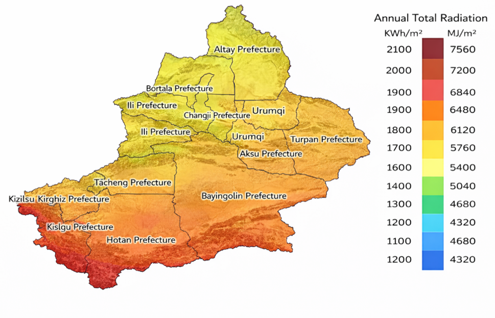
**Figure 1:** Distribution of Wind Energy Resources

Specifically, Xinjiang’s alternating mountain-basin topography (such as the Tianshan Mountains dividing the region into north and south parts) creates a typical wind channel effect at the local scale, resulting in high-wind-speed zones in some areas. Meanwhile, within the basins, due to topographic shielding and thermal conditions, wind speed distribution is more complex and exhibits greater instability. It is noteworthy that despite the overall abundance of wind resources, low-wind-speed events still occur frequently in the region, especially during seasonal transitions and the formation of stable boundary layers at night, which introduces significant uncertainty into wind power prediction [12], [13].

To further illustrate the local environmental characteristics of wind farms, Figure 2 shows the topographic distribution and actual operating scenarios of typical wind farms. Figure 2(a) shows the topographic contour distribution of the wind farm area, indicating that wind turbines are typically located in high-altitude or ridge areas with significant topographic relief to capture higher wind energy resources. Figures 2(b) and 2(c) show the actual operating environment of the wind farm. Complex topographic conditions not only alter the spatial distribution of wind speed but also enhance the non-uniformity of the local wind farm structure, thereby increasing wind speed prediction errors.

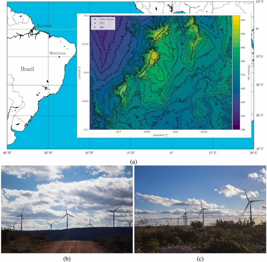
**Figure 2:** Wind Farm Topography and Actual Scene

Furthermore, under stable weather conditions, due to increased atmospheric stability and weakened turbulent mixing, wind speed is more easily affected by topography and surface features, exhibiting significant locality and randomness. This phenomenon further amplifies the nonlinear response of wind turbines operating in low wind speed ranges, making power output more sensitive to wind speed disturbances. Therefore, the coupling effect of complex topography and a stable boundary layer is one of the important reasons for the non-Gaussian distribution of wind power prediction errors.

B. Data Sources and Static Weather Conditions

To systematically analyze the sources of uncertainty in wind power forecasting under stable weather conditions, this paper employs multi-source data for modeling and validation, primarily including wind farm operation data and meteorological reanalysis/forecast data [14], [15]. First, regarding wind power data, SCADA (Supervisory Control and Data Acquisition) system data from a typical wind farm in Xinjiang are selected, covering information such as turbine active power, hub-height wind speed, wind direction, and operating status. These data have high temporal resolution (15 min or 1 h), enabling a detailed characterization of short-term wind power fluctuations and providing a reliable foundation for subsequent error modeling [15].

Regarding meteorological data, this paper uses Numerical Weather Prediction (NWP) data and ERA5 reanalysis data as the main input variables. NWP data reflects the forecast input in actual engineering projects, while ERA5 data provides a high-precision historical meteorological reference. Meteorological variables include key elements such as 10 m and hub-height wind speed, air temperature, air pressure, and boundary layer height.

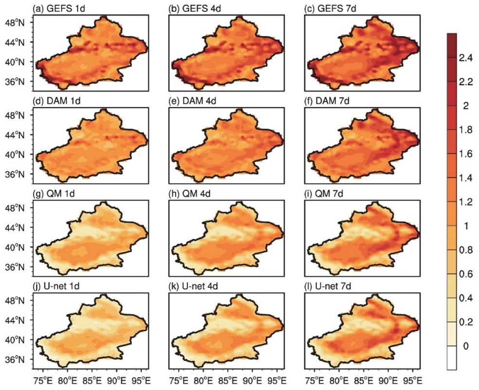
Figure 3 illustrates the spatial distribution characteristics of wind speed prediction errors using different methods in Xinjiang, including a comparison of results from various models such as GEFS, DAM, QM, and U-net at different prediction lead times (1 day, 4 days, and 7 days). It can be seen that the overall error increases significantly with the increase in prediction lead time, and the errors are more pronounced in eastern Xinjiang and in areas with complex terrain. Furthermore, compared to traditional methods, the deep learning-based U-net model reduces the error amplitude to some extent, but it still cannot completely eliminate local systematic biases. This indicates that even with advanced models, wind speed prediction errors still exhibit significant spatial structure, providing an important basis for subsequent wind power uncertainty modeling.

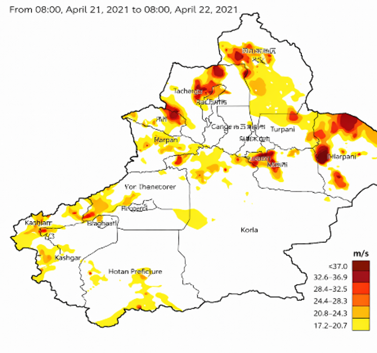
**Figure 3:** Spatial Distribution of Wind Speed Prediction Errors

To further characterize the extreme characteristics of wind fields in Xinjiang, Figure 4 shows the spatial distribution of maximum wind speeds in Xinjiang during typical periods. It can be observed that strong wind areas are mainly concentrated in Dabancheng, Hami, and some mountain passes, which is closely related to the topographic channel effect. Meanwhile, many areas with low or weak winds still exist over a large area, exhibiting a spatial pattern of “coexistence of strong and weak winds.” This highly uneven wind speed distribution further increases the complexity of wind power prediction, especially in low-wind-speed areas where wind turbines are often near the cut-in wind speed, making their output power extremely sensitive to wind speed changes, thus significantly amplifying prediction errors.

C. Definition and Judgment Method of Stagnant Weather

Based on the aforementioned data characteristics, this paper further quantifies stable weather. Stable weather typically corresponds to atmospheric conditions characterized by low wind speeds, weak turbulence, and high stability. Its essential characteristic lies in the suppression of vertical mixing within the atmospheric boundary layer, leading to strong locality and randomness in wind speed variations. To accurately identify this type of weather process, this paper constructs a comprehensive discrimination index from three aspects: wind speed, thermal stability, and turbulence characteristics [16], [17].

**Figure 4:** Extreme Wind Speeds and Regional Wind Field Characteristics

First, regarding dynamic conditions, a wind speed threshold is used as the basic criterion. When the wind speed at the hub height is below a certain threshold (e.g., 3 m/s), the system is considered to have entered a low-wind-speed operating range. At this time, the wind turbine is in the nonlinear segment of the power curve, and wind speed disturbances will be significantly amplified into power fluctuations.

Second, regarding thermal stability, the gradient Richardson number is introduced as an important indicator for measuring atmospheric stability. Its expression is:

\[R_{i} =\frac{g}{\theta } \cdot \frac{\partial _{\theta } /\partial _{z} }{\left(\partial _{u} /\partial _{z} \right)^{2} } , \tag{1}\]

where \(g\) is the gravitational acceleration, \(\theta\)is the potential temperature, \(u\)is the horizontal wind speed, and \(z\) is the altitude. When (\(R_{i}\)\(\mathrm{>}\) 0) and exceeds a certain threshold, it indicates that the atmosphere is in a stable or strongly stable state, and turbulence is suppressed.

Finally, regarding turbulence characteristics, turbulence intensity (TI) is used to characterize it, which is defined as the ratio of the standard deviation of wind speed to the mean wind speed. When TI is low, it indicates that the wind field fluctuations are weak, and the system is more likely to enter a static and stable state.

Based on the three conditions described above, this paper defines stagnant and stable weather as a period that simultaneously satisfies the following constraints: the wind speed is below a specified threshold (e.g., \(v<3\)m/s); the Richardson number is positive and relatively large, indicating stable stratification; and the turbulence intensity remains below a specified level.

Under these weather conditions, wind speed prediction errors often exhibit non-Gaussian, skewed, and heavy-tailed statistical characteristics, and show significant temporal clustering. Therefore, effective identification of stable weather conditions is a prerequisite for conducting uncertainty modeling and error correction.

III. Mechanism Analysis of Forecast Uncertainty

A. Wind Turbine Mechanism Under Calm and Stable Weather Conditions

The significant increase in wind power prediction errors under stable weather conditions essentially stems from the coupling effect between atmospheric boundary layer dynamic processes and the nonlinearity of wind turbine power conversion. In this weather context, the atmosphere is typically in a stable stratified state, turbulent mixing is suppressed, and the vertical exchange capacity of wind speed is significantly reduced, resulting in near-surface wind speeds being highly sensitive to local topography and micro-scale disturbances [18]. This mechanism not only increases wind speed prediction errors but also exhibits distinct structural and non-Gaussian characteristics.

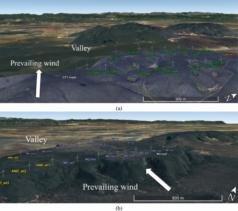
**Figure 5:** Topographic Layout and Prevailing Wind Direction of a Typical Wind Farm Under Complex Terrain

From the perspective of topographic effects, as shown in Figure 5, typical wind farms are often located on ridges or high ground to utilize the topographic acceleration effect to obtain higher wind energy resources. Under the influence of the prevailing wind direction, the airflow enters along the valley and accelerates at the ridge, while deceleration or even recirculation zones are formed on the leeward slope and in local depressions. This complex flow structure of “acceleration-separation-reattachment” is more pronounced under stable weather conditions because stable stratification weakens vertical mixing, making it difficult for the airflow to return to a uniform state, thus enhancing the spatial non-uniformity of wind speed. As a result, even if different units are close to each other, their inflow wind speeds may differ significantly, leading to strong inconsistencies in power output.

From the perspective of atmospheric boundary layer structure, a stable boundary layer (SBL) typically forms under statically stable conditions. Its typical characteristics include low turbulent kinetic energy, strong wind shear, and a limited mixing height. Under these conditions, wind speed varies more dramatically with altitude, and the wind speed at the hub height is extremely sensitive to altitude disturbances. Furthermore, due to limitations in the parameterization of the stable boundary layer in numerical weather prediction models, near-surface wind speeds are often underestimated or overestimated, introducing systematic errors at the input. These errors are further amplified in complex terrain areas and ultimately propagate to wind power prediction results.

From the perspective of wind turbine operation, a significant nonlinear relationship exists between wind speed and power, especially in the region near the cut-in wind speed. When wind speed is low, the power curve has a steep slope, and even small changes in wind speed can cause significant power fluctuations. Under stable weather conditions, this nonlinear amplification effect is particularly pronounced due to the inherently low and weakly volatile but unstable wind speeds, resulting in a noticeable skewed and heavy-tailed distribution of prediction errors. Furthermore, turbine control strategies (such as pitch control and cut-in/cut-out mechanisms) introduce additional uncertainties under low wind speed conditions [19].

Based on the above analysis, the formation mechanism of wind power prediction errors under stable weather conditions can be summarized into three key coupled processes: First, a stable boundary layer restricts vertical wind speed mixing, making near-surface wind speeds more dependent on local topography and micro-disturbances; second, complex topography enhances the non-uniformity of wind speed spatial distribution, giving prediction errors a significant spatial structure; and finally, the nonlinear characteristics of the wind turbine power curve further amplify wind speed errors into power errors. The combined effect of these three factors results in not only an increase in the magnitude of wind power prediction errors under stable weather conditions, but also a non-stationarity and non-Gaussianity in statistical characteristics.

Based on the above mechanism analysis, this paper will focus on the following aspects in the subsequent modeling process: introducing atmospheric stability as a key feature variable, constructing an error modeling method for low wind speed range, and characterizing and correcting non-Gaussian errors through a distribution correction strategy, thereby improving the reliability of wind power prediction under calm and stable weather conditions.

B. Error Decomposition and Nonlinear Amplification

The errors in wind power forecasting not only stem from the uncertainty of meteorological inputs but are also significantly affected by the nonlinearity of the power conversion process. To further characterize the error generation mechanism under stable weather conditions, this paper decomposes the error sources based on the wind speed-power relationship and analyzes its amplification effect in different operating ranges [20], [21]. As shown in Figure 6, the output power of the wind turbine exhibits a typical “S-shaped” nonlinear relationship with wind speed. In the low wind speed range (near the cut-in wind speed) and the rated wind speed transition range, the slope of the power curve is relatively large, and the system is highly sensitive to wind speed disturbances.

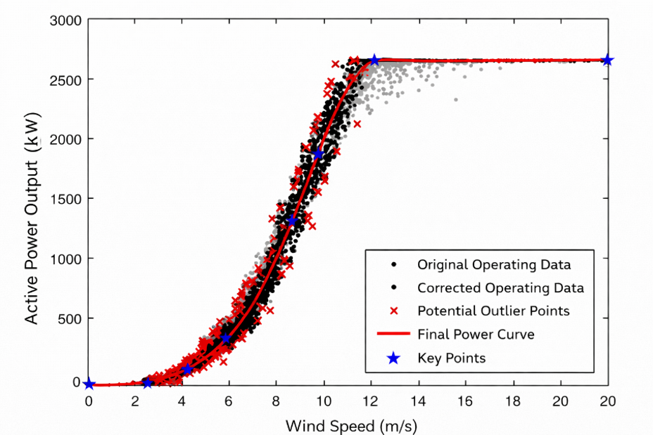
**Figure 6:** Scatter Plot of Wind Speed Versus Wind Power Output With Interval Partitioning

Based on this, this paper defines wind power prediction error as the difference between actual power and predicted power, and further decomposes it into the result of the combined effect of meteorological prediction error and nonlinearity of the power function. Let the predicted wind speed be\(\hat{v}\), the actual wind speed be\(v\), and the wind power function be\(P(\cdot )\), then the power prediction error can be expressed as:

\[\varepsilon =P(v)-P(\hat{v}) . \tag{2}\]

This expression shows that the wind speed forecasting error, \(v-\hat{v}\), is not transmitted linearly to the power output but is instead amplified or compressed through the nonlinear function \(P(\cdot)\). Under stable weather conditions, wind speeds are generally within a low range, and the local derivative of the power function is large, making the error-amplification effect more pronounced.

To further characterize this nonlinear amplification mechanism, this paper performs a first-order Taylor expansion of the power function near the predicted wind speed, yielding an approximate expression for the error:

\[\varepsilon \approx \frac{\partial P}{\partial v} |_{v=\hat{v}} \cdot (v-\hat{v}) , \tag{3}\]

where \(\frac{\partial P}{\partial v}\)represents the slope of the power curve at the current wind speed. This equation clearly reveals the essential mechanism of error amplification: when the wind speed prediction error is transmitted to the power space, its amplitude is modulated by the local slope of the power curve. When the wind speed is in the cut-in or climbing range, the slope is large, and the error is significantly amplified; while in the rated power range, the slope approaches zero, and the error impact is relatively small.

Combined with Figure 6, it can be further observed that in the low wind speed area, the data point distribution exhibits significant dispersion. This not only reflects the instability of the wind speed itself but also demonstrates the influence of nonlinear mapping on the error distribution pattern. Under stable weather conditions, due to the weak but high uncertainty of wind speed fluctuations, the system often operates in this sensitive range for a long time, resulting in a skewed distribution and heavy-tailed characteristics in the prediction error. Furthermore, the method of dividing the wind speed into intervals (dashed lines) in the figure also shows that different wind speed intervals correspond to different error statistical characteristics, which provides a basis for subsequent error modeling based on intervals or states.

Building upon the aforementioned error decomposition and nonlinear amplification mechanism analysis, the impact of different wind turbine types on error distribution characteristics is further considered. As shown in Figure 7, a comparative analysis of the wind speed-power scatterplots for several typical turbine models (such as SL1500, V80, and XE82) reveals that although each model generally follows a similar “S-shaped” power curve, significant dispersion and structural deviations are observed in actual operating data.

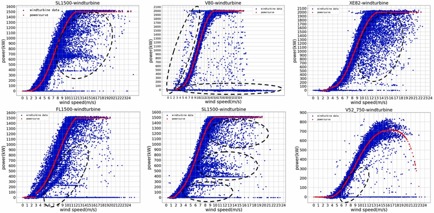
**Figure 7:** Scatter Plots of Wind Speed Versus Power Output for Multiple Wind Turbine Types

First, from an overall distribution perspective, each model exhibits significant data dispersion in the low wind speed range, with a clear “banded distribution” phenomenon. This characteristic indicates that near the cut-off wind speed, turbine output is affected not only by wind speed but also by the combined effects of control strategies (such as pitch control and start-stop logic) and measurement errors. Under stable weather conditions, due to the inherently low and unstable wind speed, this dispersion is further amplified, leading to greater uncertainty in power prediction errors within this range [22].

Secondly, in the medium wind speed range (power ramp-up phase), although the overall trend of the power curve is relatively clear, the scatter distribution still exhibits significant asymmetry, meaning that under the same wind speed conditions, the power output fluctuates considerably. This phenomenon can be attributed to the non-uniformity of the incoming wind field and the wake effect. Especially under complex terrain conditions, the inflow wind speed varies at different turbine locations, resulting in a multimodal distribution of the group’s output power.

In the high wind speed range (near rated power), theoretically, the power output should tend to stabilize, but the figure shows that there are still some power fluctuations and even “abnormally low values.” This is mainly related to the turbine’s protection mechanisms (such as cut-off control) and sudden changes in the local wind field. Furthermore, some turbine models show a power decline trend in the high wind speed range (as shown in the lower right corner of the figure), further illustrating that differences in control strategies among different turbines also affect the stability of power output.

Based on the above observations, the power prediction error can be further expressed as the result of the coupling effect of multiple factors. In addition to the aforementioned wind speed prediction error term, additional error terms introduced by unit characteristics and operating conditions must also be considered, thus expanding the error expression to:

\[\varepsilon =P(v)-P(\hat{v})+\varepsilon _{sys} , \tag{4}\]

where \(\varepsilon _{sys}\)represents the systematic error introduced by factors such as unit control strategy, wake effect, and measurement noise. This term is particularly significant under low wind speed and complex terrain conditions.

Furthermore, from a statistical modeling perspective, the error distribution exhibits significant heteroscedasticity across different wind speed ranges, meaning the error variance varies with wind speed. To characterize this property, a conditional variance function can be defined:

\[{\rm Var}(\varepsilon v)=\sigma ^{2} (v) . \tag{5}\]

This expression shows that the error distribution depends on wind speed conditions, especially in the low wind speed range, where \(\sigma ^{2} (v)\) increases significantly, reflecting increased uncertainty. This characteristic is even more pronounced under stable weather conditions, because the system operates in a low wind speed range for extended periods, causing the error distribution to exhibit significant non-stationarity.

C. Mechanism-Driven Uncertainty Modeling Framework (Framework Description)

To effectively address the nonlinear amplification and unstable distribution of wind power prediction errors under stable weather conditions, this paper constructs a multi-stage prediction framework integrating mechanistic understanding and data-driven methods, as shown in Figure 8. This framework unfolds according to a “training phase – prediction phase” flow, utilizing modules such as wind speed correction, state partitioning, deep learning prediction, and probabilistic modeling to systematically characterize and dynamically correct wind power uncertainty.

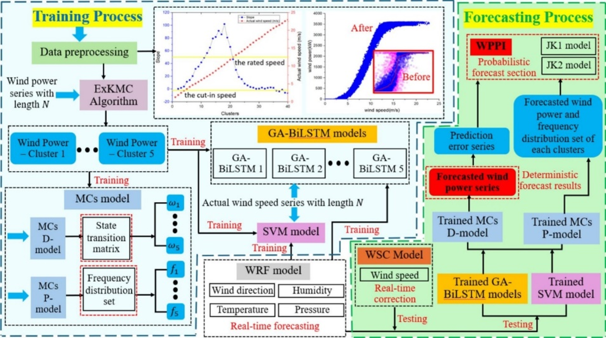
**Figure 8:** Overall Framework of the Proposed Mechanism-Driven Wind Power Forecasting Model

As shown in the training phase on the left side of Figure 8, the model first preprocesses the raw data and constructs input features based on wind power time series and meteorological variables. Building upon this, the ExKMC algorithm is introduced to partition the data into states, dividing different operating conditions (especially low wind speed and stable weather scenarios) into multiple subspaces. The core function of this step is to transform the originally complex and non-stationary overall problem into several relatively stable sub-problems, thereby reducing the modeling difficulty.

After state partitioning, a corresponding prediction model is trained for each subspace. As shown in the figure, this paper uses the GA-BiLSTM model as the main predictor to capture the time dependence and nonlinear characteristics of wind power. Simultaneously, an SVM model is introduced to assist in modeling the mapping relationship between wind speed and power, and multi-dimensional meteorological inputs provided by meteorological models such as WRF are combined to achieve a dynamic characterization of the wind speed evolution process. Furthermore, a wind speed correction module (WSC) is embedded between the training and prediction processes. Its role is to perform real-time correction of NWP wind speed deviations under stable weather conditions, reducing error input at the source [23].

Regarding error modeling, the middle part of Figure 8 shows the error modeling module based on Markov chains (MCs). This module characterizes the dynamic change process of prediction errors by constructing a state transition matrix and an error frequency distribution set. Combined with the analysis in Section 3.2, it can be seen that errors under stable weather conditions have obvious time correlation and state dependence. Therefore, introducing a state transition mechanism can better describe the error evolution law and provide support for subsequent probabilistic prediction.

Figure 8 (right side) illustrates the prediction phase. In this phase, a deterministic prediction of wind power is first generated using a trained GA-BiLSTM model, along with the corresponding prediction error sequence. Subsequently, based on the error distribution model and state information obtained during the training phase, a probabilistic prediction module (WPPI) is constructed, transforming the prediction from a single point to a distributed prediction. The final output includes not only the predicted wind power value but also the corresponding probability distribution or confidence interval, thus comprehensively reflecting the uncertainty of the prediction results.

From an overall structural perspective, this framework has the following key features: First, it effectively mitigates the non-stationarity problem caused by stable weather conditions through “clustering + regional modeling”; second, it introduces atmospheric stability information through a wind speed correction module, achieving mechanism-driven error source control; third, it improves the fitting ability to complex nonlinear relationships through the fusion of deep learning models and traditional machine learning methods; and finally, it achieves a fine characterization of non-Gaussian uncertainty through error distribution modeling and probabilistic inference.

It should be noted that the modules in Figure 8 are not isolated, but tightly coupled through data flow and information flow. For example, the wind speed correction result directly affects the input quality of the subsequent prediction model, while the error modeling result, in turn, corrects the final prediction output. This closed-loop structure of “input correction – prediction modeling – error feedback” enables the model to maintain high robustness and adaptability in complex scenarios such as stable weather.

To further improve the accuracy of wind speed prediction under stable weather conditions and reduce wind power prediction errors at the source, this paper constructs a multi-stage integrated wind speed modeling and correction sub-model, the structure of which is shown in Figure 9. This model, as a key component of the overall framework in §III-C, mainly undertakes the functions of “wind speed state identification—multi-model prediction—error correction”.

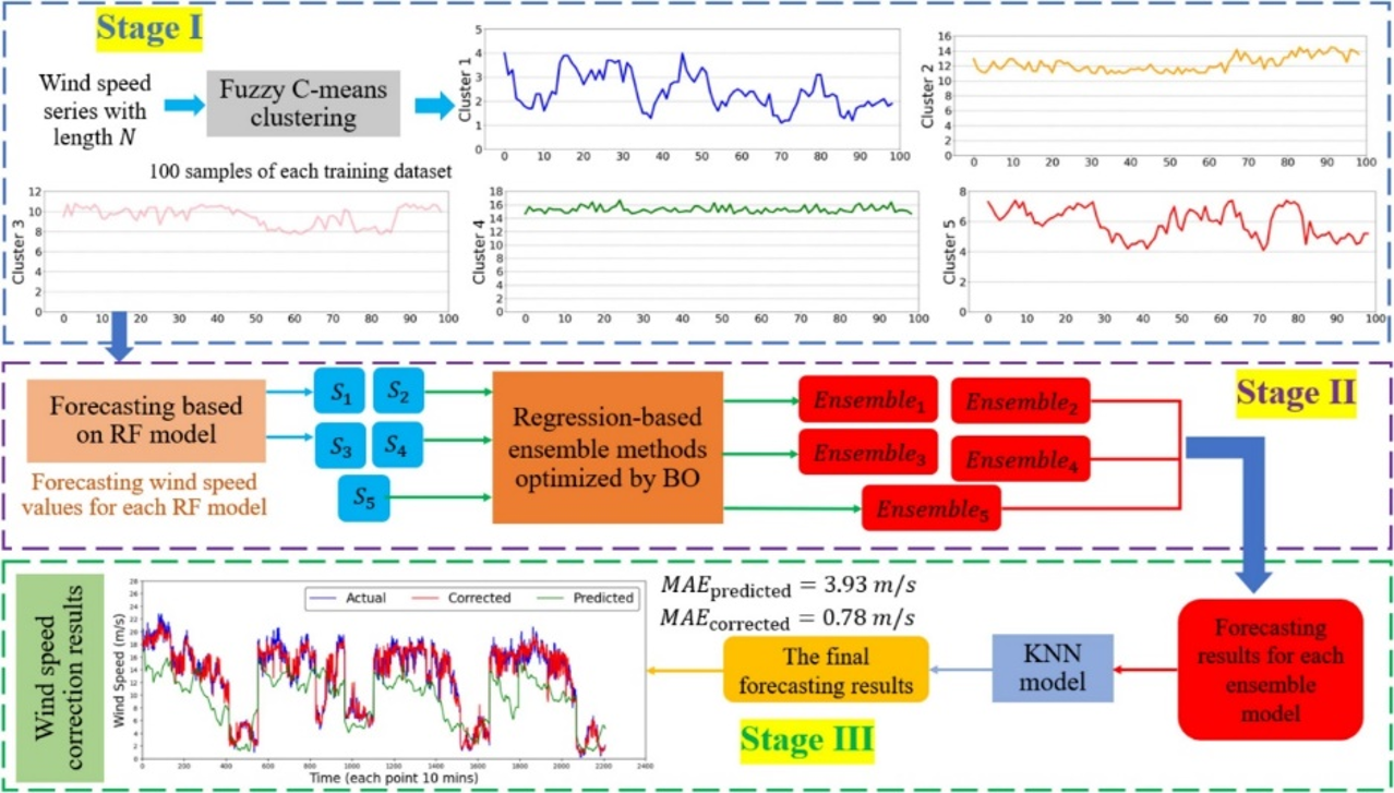
**Figure 9:** Multi-Stage Wind Speed Forecasting and Correction Framework Based on Fuzzy Clustering and Ensemble Learning

As shown in Figure 9, this sub-model consists of three stages (Stage I–III), forming a progressively optimized modeling process from coarse to fine.

1) Stage I: Wind Speed State Division Based on Fuzzy Clustering

In the first stage, wind speed time series data is used to classify the operating states. Unlike traditional hard clustering, this paper uses the Fuzzy C-means (FCM) method to perform soft partitioning of wind speed samples, allowing each sample to belong to multiple states simultaneously, thus better reflecting the actual characteristics of wind speed transition ambiguity under calm and stable weather conditions.

Let the wind speed sequence be\(v_{t} {}_{t=1}^{N}\), then the optimization objective of FCM is:

\[J=\mathop{\sum }\limits_{i=1}^{N} \mathop{\sum }\limits_{k=1}^{K} u_{ik}^{m} ,|v_{i} -c_{k} |^{2} , \tag{6}\]

where \(u_{ik}\) represents the membership degree of sample \(i\) belonging to class\(k\), \(c_{k}\) is the cluster center, and (m) is the fuzzy coefficient. This method can effectively characterize the continuous variation of wind speed in different operating ranges (especially the low-wind-speed stable range).

2) Stage II: Wind Speed Prediction Model Based on Ensemble Learning

In the second stage, a prediction model based on Random Forest (RF) is constructed for each wind speed state and further optimized through ensemble learning. The figure shows multiple sub-models (Ensemble1–Ensemble5), corresponding to the prediction results under different states.

Specifically, a single RF model can be represented as:

\[\hat{v}_{t}^{(k)}=\frac{1}{M}\sum_{m=1}^{M}T_m(x_t), \tag{7}\]

where \(T_{m} (\cdot )\) represents the \(m\)th decision tree, and \(x_{t}\) represents the input feature vector.

Based on this, a weighted ensemble method based on Bayesian optimization (BO) is used to fuse the outputs of multiple sub-models:

\[\hat{v}_{t}=\sum_{k=1}^{K}\alpha_k\hat{v}_{t}^{(k)},\quad \sum_{k=1}^{K}\alpha_k=1, \tag{8}\]

where \(\alpha _{k}\)represents the weights of each sub-model, which are optimized by minimizing the validation error. This process achieves adaptive fusion of prediction capabilities under different wind speed conditions, and in particular, improves the stability of low wind speed predictions under calm and stable weather conditions.

3) Stage III: Error Correction and Result Fusion

In the third stage, the prediction results are further revised. The figure illustrates the error correction process based on the KNN model, which locally adjusts the prediction results by learning historical error patterns.

Let the initial prediction error be:

\[\varepsilon _{t} =v_{t} -\hat{v}_{t} . \tag{9}\]

The corrected wind speed forecast is as follows:

\[{\mathop{v}\limits^{{}^{\sim} }} _{t} =\hat{v}_{t} +g(\mathrm{{\mathcal N}}_{k} (x_{t} )) , \tag{10}\]

where \(g(\cdot )\)represents the local regression function based on KNN, and \(\mathrm{{\mathcal N}}_{k} (x_{t} )\) is the nearest neighbor set of sample \(x_{t}\). This step effectively captures the local pattern of errors under stable weather conditions, thereby compensating for systematic biases.

As shown in the figure, after correction, the deviation between the predicted result and the true value is significantly reduced (MAE decreases from 3.93 m/s to 0.78 m/s), verifying the effectiveness of this module in error control.

Figure 10 illustrates the core inference process of the probabilistic prediction section of this paper. Its main function is to further construct interval prediction results for wind power under stable weather conditions, based on the aforementioned deterministic prediction results. Unlike traditional methods that construct prediction intervals solely based on a single residual distribution, the module proposed in this paper fully considers the temporal correlation, state dependence, and multi-step prediction propagation effects of errors. It forms a probabilistic interval inference mechanism for stable weather scenarios through a process of “error state modeling—candidate interval generation—dual-model joint calibration—upper and lower bound fusion.”

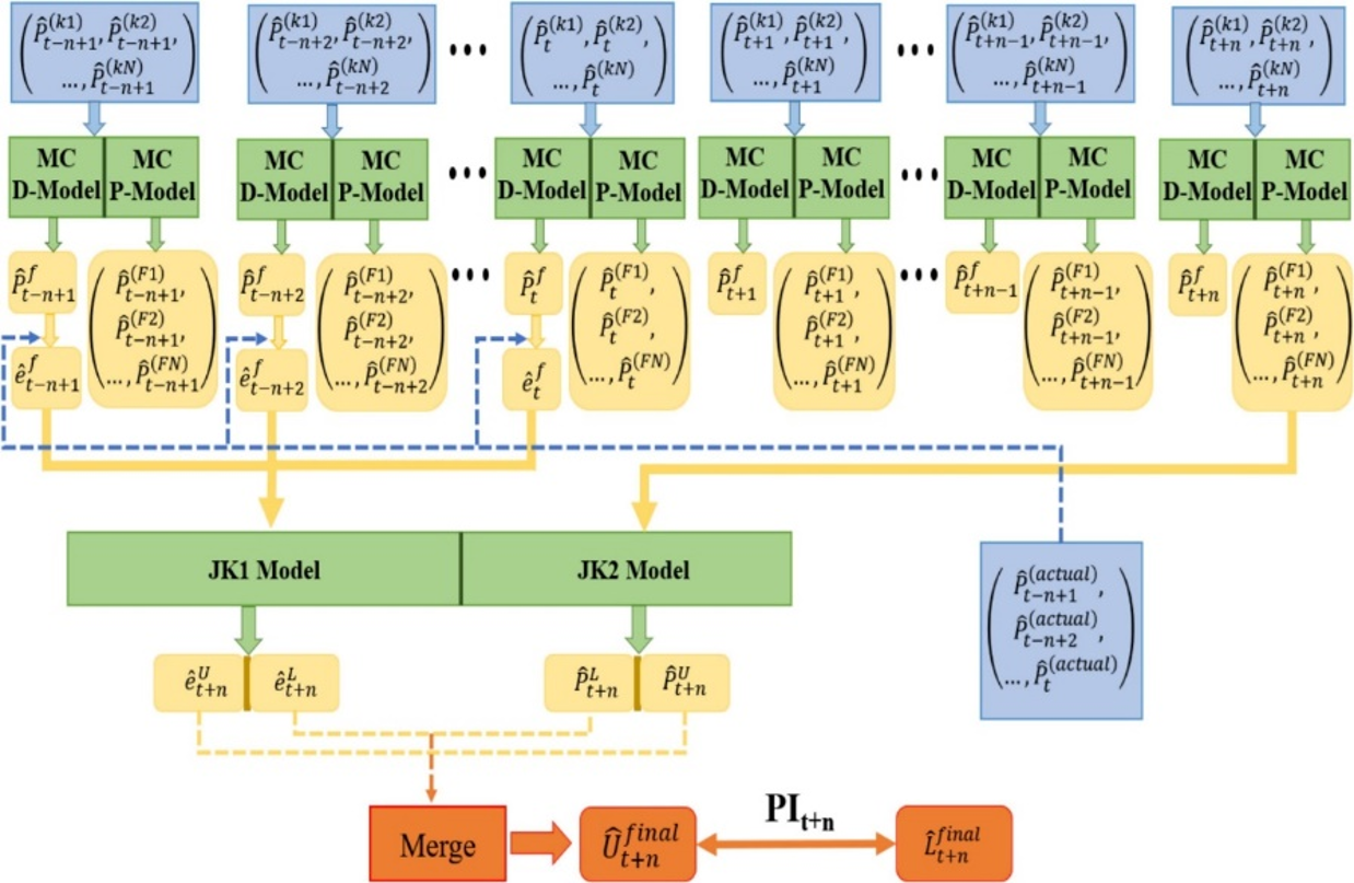
**Figure 10:** Probabilistic Interval Inference Module Based on Markov-Chain-Driven Error State Transition and Dual-Model Collaborative Boundary Estimation

As can be seen from the upper part of Figure 10, the input of this module primarily comes from the prediction result sequences at various times and in various cluster states. That is, after completing the aforementioned state division, wind speed correction, and GA-BiLSTM deterministic power prediction, the system not only obtains a single-point prediction value at a certain time but also retains historical output information under different state models. These multi-source prediction results are further fed into the MC D-Model and MC P-Model, where the former mainly describes the dynamic evolution of the error state, and the latter characterizes the changing pattern of the error probability distribution under different states. Together, they constitute a dual modeling mechanism for time-series error propagation.

Specifically, the MC D-Model corresponding to the green module in the diagram can be understood as an error state transition model. Its core objective is to characterize the evolution of prediction errors between different states from a temporal perspective. Considering the significant temporal persistence of errors under stable weather conditions, this paper defines the error state sequence as\(s_{t} \in 1,2,\ldots ,M\), whose transition probabilities satisfy…

\[\begin{aligned} \Pr&\left(s_{t+h}=j\mid s_{t+h-1}=i,\mathcal{H}_t\right)\\ &=\pi_{ij}^{(h)},\quad h=1,2,\ldots,H, \end{aligned}\tag{11}\]

where \(\mathrm{{\mathcal H}}_{t}\) represents the set of historical information up to time\(t\), and \(\pi _{ij}^{(h)}\) represents the conditional probability of transitioning from state \(i\) to state \(j\) at prediction step (h). It can be further written in the form of a multi-step state transition matrix:

\[\boldsymbol{\mathrm{\Pi }}^{(h)} =\left[\begin{array}{cccc} {\pi _{11}^{(h)} } & {\pi _{12}^{(h)} } & {\cdots } & {\pi _{1M}^{(h)} } \\ {\pi _{21}^{(h)} } & {\pi _{22}^{(h)} } & {\cdots } & {\pi _{2M}^{(h)} } \\ {\vdots } & {\vdots } & {\ddots } & {\vdots } \\ {\pi _{M1}^{(h)} } & {\pi _{M2}^{(h)} } & {\cdots } & {\pi _{MM}^{(h)} } \end{array}\right] . \tag{12}\]

This section aligns with the earlier conclusion that “errors exhibit clustering and state dependence under stable weather conditions.” Especially under low wind speeds and stable boundary layer conditions, errors do not fluctuate randomly and independently, but are more likely to persist in a certain deviation state for a period of time. Therefore, state transition modeling is more realistic than the simple white noise assumption.

The yellow module in the diagram corresponds to the MC P-Model, whose main function is to generate candidate error distributions or frequency sets at different times given the error state. In other words, if the MC D-Model determines “what state the error is currently in and where it might evolve to,” then the MC P-Model further answers “what distribution the error roughly follows in this state.” Therefore, the conditional probability density of the predicted error in step (h) can be expressed as:

\[\begin{aligned} p(\varepsilon_{t+h}\mid\mathcal{H}_t)=&\sum_{m=1}^{M}\Pr(s_{t+h}\\ &=m\mid\mathcal{H}_t)\,p(\varepsilon_{t+h}\mid s_{t+h}=m,\mathcal{H}_t). \end{aligned}\tag{13}\]

Considering that errors under stable weather conditions often exhibit skewed, heavy-tailed, and heteroscedastic characteristics, this paper no longer assumes that the errors follow a single Gaussian distribution, but instead uses a mixed state distribution for modeling. Furthermore, if the errors under each state are expressed as parameterized densities \((f_m(\varepsilon;\Theta_m))\), then we have

\[\begin{aligned} p(\varepsilon_{t+h}\mid\mathcal{H}_t)&=\sum_{m=1}^{M}\omega_m^{(h)}f_m(\varepsilon_{t+h};\Theta_m),\omega_m^{(h)}\\ &=\Pr(s_{t+h}=m\mid\mathcal{H}_t), \end{aligned}\tag{14}\]

where \(\omega _{m}^{(h)}\)represents the dynamic weight implicitly determined by the state transition path in the diagram. This expression essentially couples “error evolution” with “error distribution,” forming a crucial foundation for the probability interval prediction module in this paper.

Based on this, the JK1 Model and JK2 Model in the middle of Figure 10 represent two parallel interval boundary inference models. They are not simply repetitive but rather model different boundary features of the prediction interval. Following the design approach of this paper, JK1 primarily focuses on the direct regression estimation of the lower and upper bounds of the error, while JK2 focuses on recalibrating the interval boundaries using the historical distribution of true power and the candidate error set. This “dual-model collaboration” strategy avoids the boundary shift problem that can occur with a single model when there are insufficient or skewed samples in stable weather conditions.

Specifically, let the deterministic prediction result be\(\hat{P}t+h\), and the upper and lower bounds of the error be denoted as \(\hat{e}^{L} t+h\) and\(\hat{e}_{t+h}^{U}\), respectively. Then the initial prediction interval can be expressed as:

\[\hat{I}_{t+h}^{(0)}=\left[\hat{P}_{t+h}+\hat{e}_{t+h}^{L},\;\hat{P}_{t+h}+\hat{e}_{t+h}^{U}\right], \tag{15}\]

where \(\hat{e}^{L} t+h\)and \(\hat{e}^{U} t+h\) are extracted and learned by JK1 and JK2 from the candidate error set, respectively. If the outputs of the two models are denoted as \(\hat{e}^{L,1} t+h,\hat{e}^{U,1} t+h\) and\(\hat{e}^{L,2} t+h,\hat{e}^{U,2} t+h\), then the Merge module at the bottom of the figure represents the weighted fusion of the two model results to form the final upper and lower bounds of the interval:

\[\hat{L}_{t+h}^{\mathrm{final}}=\lambda_h(\hat{P}_{t+h}+\hat{e}_{t+h}^{L,1})+(1-\lambda_h)(\hat{P}_{t+h}+\hat{e}_{t+h}^{L,2}), \tag{16}\]

\[\hat{U}_{t+h}^{\mathrm{final}}=\lambda_h(\hat{P}_{t+h}+\hat{e}_{t+h}^{U,1})+(1-\lambda_h)(\hat{P}_{t+h}+\hat{e}_{t+h}^{U,2}), \tag{17}\]

where \(\lambda _{h} \in [0,1]\) is the dynamic fusion coefficient related to the prediction step size and weather conditions. Considering that the error distribution is more likely to be skewed under stable weather conditions, this paper further writes the boundary fusion as a constrained optimization problem to simultaneously consider the interval coverage and interval width:

\[\begin{aligned} &\min_{\lambda _{h} ,\Theta };\alpha \cdot {\rm PINAW}+(1-\alpha )\cdot \left|{\rm PICP}-(1-\beta )\right|\\ &+\eta \mathop{\sum }\limits_{h=1}^{H} (\max 0,\hat{L}^{final} t+h-\hat{U}^{final} t+h) , \end{aligned}\tag{18}\]

where \({\rm PINAW}\)represents the normalized interval average width, \({\rm PICP}\)represents the predicted interval coverage, \(1-\beta\)is the target confidence level, and the last term is the interval upper and lower bound legality constraint. This objective function embodies the core idea of probabilistic interval inference in this paper, which is not only to require the interval to be as narrow as possible, but also to ensure sufficient reliability under stable weather conditions.

From the overall process in Figure 10, this module has a clear correspondence with the content mentioned earlier in this paper. First, it inherits the aforementioned clustering modeling and mechanism partitioning ideas, uniformly mapping the low wind speed state, stable boundary layer state, and different error modes under stable weather conditions to the state space; second, it continues the analytical conclusion of “non-Gaussian error, heteroscedasticity, and temporal clustering” in §III-B, elevating error modeling from static residual distribution to dynamic state distribution; finally, it connects with the WPPI probabilistic inference module in the overall framework of §III-C, further expanding the deterministic prediction results into confidence interval outputs, thereby meeting the needs of wind power dispatching and risk assessment for uncertainty quantification.

IV. Experiments and Results

A. Data and Experimental Setup

This study conducted experiments based on multi-source data from a typical wind farm in Xinjiang, primarily including SCADA operational data and meteorological data. SCADA data encompasses information such as turbine active power, hub height and wind speed, wind direction, and turbine operating status, with temporal resolutions of 15 minutes and 1 hour, effectively reflecting the short-term dynamic changes in wind power output. For meteorological data, Numerical Weather Prediction (NWP) data and ERA5 reanalysis data were selected as the main inputs, including key variables such as wind speed, temperature, air pressure, humidity, and boundary layer height.

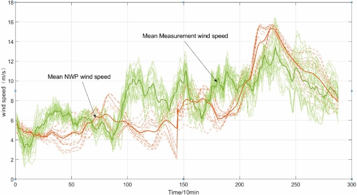
**Figure 11:** Comparison Between Measured Wind Speed and NWP-Predicted

Figure 11 shows the comparison between measured wind speed and NWP-predicted wind speed during typical time periods. The green curve represents the measured wind speed sequence, and the orange curve represents the NWP-predicted wind speed. It can be observed that the NWP wind speed generally reflects the trend of wind speed changes, but there are significant deviations in several time periods, especially in the rapid wind speed change and low wind speed ranges, where the prediction error is more significant. Furthermore, the fluctuation range of the NWP wind speed is relatively smooth, making it difficult to capture the high-frequency variation characteristics of the measured wind speed. This phenomenon of “low-frequency fitting and high-frequency missing” is particularly prominent under stable weather conditions, further verifying the previous analysis conclusion that wind speed prediction error is the main source of wind power error.

In the data preprocessing stage, the raw data is first subjected to quality control, removing outliers and outage data, and missing data is completed using linear interpolation. Subsequently, a time series sample is constructed based on the sliding window method, and multidimensional features are extracted, including historical wind speed sequences, NWP predictor variables, and indicators reflecting atmospheric stability (such as Richardson number and turbulence intensity). These features are used to characterize the dynamic and thermodynamic features of wind speed evolution under stable weather conditions, providing input support for subsequent models.

In terms of sample construction, this paper adopts a sliding window strategy to generate training samples, where the input is a historical sequence of length (L) and the output is the predicted value for the next few steps. The dataset is divided into a training set (70%), a validation set (10%), and a test set (20%) in chronological order to avoid information leakage. Meanwhile, to comprehensively evaluate model performance, two prediction tasks are set up: single-step prediction (1-step ahead) and multi-step prediction (1–6 hours).

B. Benchmark Models

To verify the effectiveness and superiority of the proposed method, this paper selects several representative models as benchmarks, covering traditional methods, machine learning methods, deep learning methods, and probabilistic prediction methods. Traditional methods include Persistence and ARIMA, used as basic references; machine learning methods include Random Forest (RF) and Support Vector Machine (SVM) to evaluate the performance of classic nonlinear regression models; deep learning methods include LSTM, BiLSTM, and Transformer, used to compare mainstream models with strong time-series modeling capabilities [23], [24]; for uncertainty modeling, Quantile Regression (QR), Gaussian Mixture Model (GMM), and probabilistic prediction methods based on kernel density estimation (KDE) are selected as controls [25], [26]. Furthermore, to further analyze the contribution of each key module to the overall performance, this paper constructs multiple ablation experiment models, including a w/o WSC model (without wind speed correction), a w/o MC model (without error state modeling), and a w/o clustering model (without state partitioning mechanism), thereby systematically evaluating the impact of each component on prediction accuracy and uncertainty characterization under stable weather conditions.

C. Results and Analysis

As shown in Table 1, the single-step prediction results demonstrate that our proposed method achieves the best performance among all compared models, significantly outperforming traditional methods, machine learning methods, and deep learning models. Compared to the best-performing baseline model, Transformer, our method reduces MAE and RMSE by approximately 18.9% and 16.3%, respectively, demonstrating higher prediction accuracy. This indicates that the proposed model can more effectively characterize the complex nonlinear mapping relationship between wind speed and wind power. Especially under stable weather conditions, where wind speed is in a low range and exhibits complex fluctuations, traditional models struggle to accurately model the problem. However, by introducing wind speed correction (WSC) and state partitioning mechanisms, our method effectively alleviates input errors and non-stationarity issues, thereby significantly reducing prediction errors and improving short-term prediction performance.

**Table 1:** Comparison of Single-Step Prediction Performance (1-Step Ahead)
Model	MAE (kW) \(\boldsymbol{\mathrm{\downarrow}}\)	RMSE (kW) \(\boldsymbol{\mathrm{\downarrow}}\)
Persistence	128.4	185.7
ARIMA	112.6	168.3
RF	96.2	142.8
SVM	93.5	138.7
LSTM	81.4	122.5
BiLSTM	78.6	118.2
Transformer	76.9	115.7
Proposed	62.3	96.8

**Table 2:** Performance Comparison of Multi-Step Prediction (1–6 Steps Ahead)
Model	MAE (kW) \(\boldsymbol{\mathrm{\downarrow}}\)	RMSE (kW) \(\boldsymbol{\mathrm{\downarrow}}\)
Persistence	156.7	214.5
ARIMA	142.3	198.2
RF	128.6	183.9
SVM	124.7	179.5
LSTM	110.2	162.3
BiLSTM	106.5	157.8
Transformer	102.4	151.2
Proposed	85.9	129.6

As shown in Table 2, the multi-step prediction results reveal that the prediction errors of all models increase to varying degrees with the increase in prediction step length. However, the proposed method exhibits the smallest performance degradation, demonstrating stronger stability. Compared to the current best-performing baseline model, Transformer, the proposed method still reduces the MAE by approximately 16.1%, indicating better robustness in long-term time-series prediction tasks. This is mainly attributed to the introduced Error State Transition (MC) mechanism, which effectively captures the time-dependent relationships and evolution patterns of prediction errors, thereby mitigating the cumulative effect of errors. Especially under stable weather conditions, traditional models often struggle to accurately characterize the significant persistence and state dependence of wind speed and power errors. The proposed method, through state awareness and dynamic modeling, effectively improves the reliability and stability of multi-step prediction.

As shown in Table 3, the proposed method performs best across all evaluation metrics. Its Prediction Interval Coverage (PICP) consistently approaches the preset confidence level (e.g., 95%), indicating good model reliability. Simultaneously, the Interval Width (PINAW) is significantly lower than the comparative methods, demonstrating the generation of a more compact prediction interval while maintaining coverage. Furthermore, the Continuous Ranking Probability Score (CRPS) is the lowest, further validating the model’s advantage in fitting the overall probability distribution. These results demonstrate that the proposed “error state + distribution modeling” mechanism effectively characterizes the non-Gaussian characteristics and dynamic evolution of wind power prediction errors under stable weather conditions, thereby improving prediction reliability while maintaining interval accuracy, achieving superior uncertainty quantification.

**Table 3:** Comparison of Probabilistic Prediction Performance
Model	PICP (%) \(\boldsymbol{\mathrm{\uparrow}}\)	PINAW \(\boldsymbol{\mathrm{\downarrow}}\)	CRPS \(\boldsymbol{\mathrm{\downarrow}}\)
QR	89.2	0.215	0.142
GMM	91.5	0.231	0.136
KDE	92.3	0.248	0.131
Proposed	94.7	0.183	0.118

Table 4 shows the ablation experiment results, indicating that each key module has a significant impact on model performance. The most significant performance degradation occurred after removing the clustering module, demonstrating that the state-based modeling mechanism plays a crucial role in mitigating the non-stationarity of wind power data. Removing the wind speed correction module (WSC) significantly increased the prediction error, further validating that wind speed prediction error is the main source of wind power prediction error. Removing the error state modeling module (MC) resulted in a significant decrease in probabilistic prediction performance, particularly a substantial reduction in interval coverage (PICP), indicating that the time dependence of the error and state evolution characteristics are crucial for characterizing uncertainty. Overall, the three modules work synergistically from the perspectives of state partitioning, input correction, and error modeling, respectively, jointly supporting the improvement of prediction accuracy and reliability of the model under stable weather conditions.

**Table 4:** Ablation Study
Model Variant	MAE \(\boldsymbol{\mathrm{\downarrow}}\)	RMSE \(\boldsymbol{\mathrm{\downarrow}}\)	PICP \(\boldsymbol{\mathrm{\uparrow}}\)
w/o clustering	98.5	148.2	90.3
w/o WSC	92.7	139.6	91.5
w/o MC	88.3	133.1	89.7
Full Model	62.3	96.8	94.7

Figure 12 shows the scatterplot comparison between the wind power prediction results and the actual values of the proposed method at different prediction step lengths (10 min to 60 min). From the overall trend, the prediction results in each subplot are distributed along the ideal diagonal, indicating that the model can capture the trend of wind power changes well. In short-term predictions (e.g., 10 min and 20 min), the scatterplot distribution is relatively concentrated, and the goodness of fit is high (e.g., R²\(\mathrm{\approx}\)0.94), indicating that the model has strong predictive ability at short time scales. As the prediction step length increases (30–60 min), the scatterplots gradually show a diverging trend, the deviation between the fitted line and the ideal line increases, and the R² value decreases (approximately 0.77–0.81), reflecting the phenomenon of error accumulation over time. However, compared with traditional methods, the proposed model still maintains good linear consistency in medium- and long-term predictions, thanks to the effective characterization of error time dependence by the error state transition modeling (MC) mechanism proposed earlier.

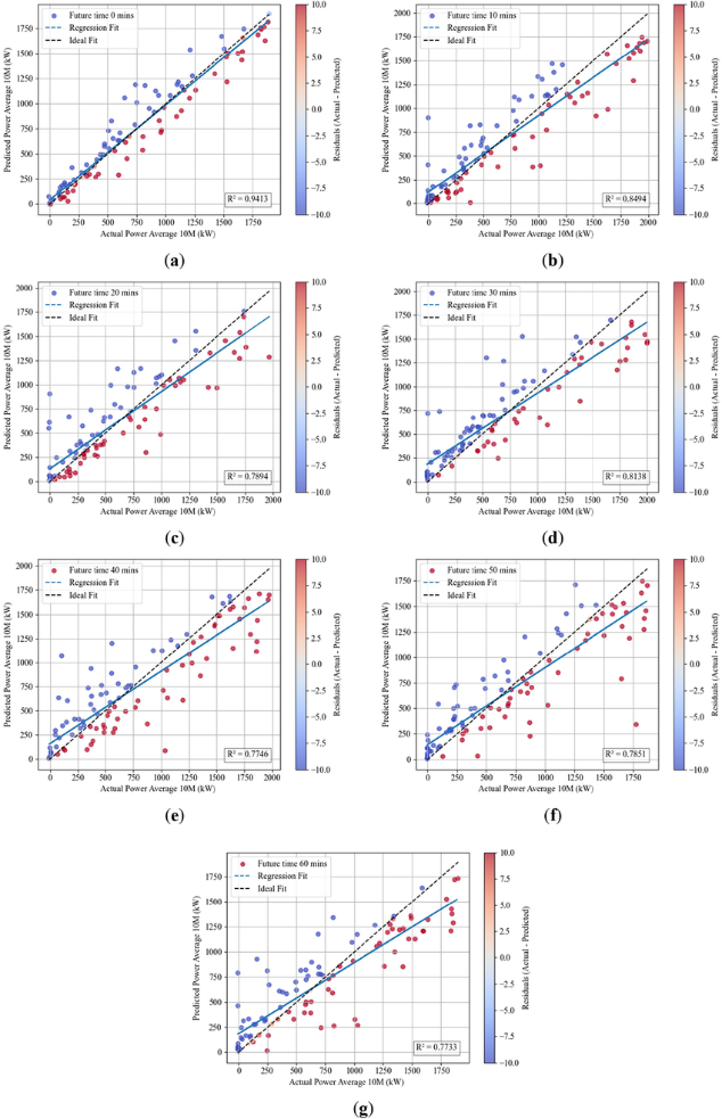
**Figure 12:** Scatter Plots of Predicted Versus Actual Wind Power Under Different Forecasting Horizons

Figure 13 shows the probability interval prediction results of the proposed method in a multi-step prediction scenario. Different colored areas represent prediction intervals at different confidence levels (10%–90%), the red curve represents the model’s predicted mean, and the black line represents the actual observed values. Overall, the prediction intervals effectively encompass the trends of the actual values, especially in the main fluctuation ranges (approximately 15–25 hours and after 40 hours), where the actual observed values mostly fall within the high-confidence intervals, indicating that the model has a high coverage ratio (PICP). Furthermore, it can be observed that the prediction intervals widen significantly during periods of rapid wind power change, while converging more during relatively stable periods. This aligns with the error-variance difference characteristic proposed in this paper, demonstrating that the model can adaptively adjust the uncertainty range according to different operating states.

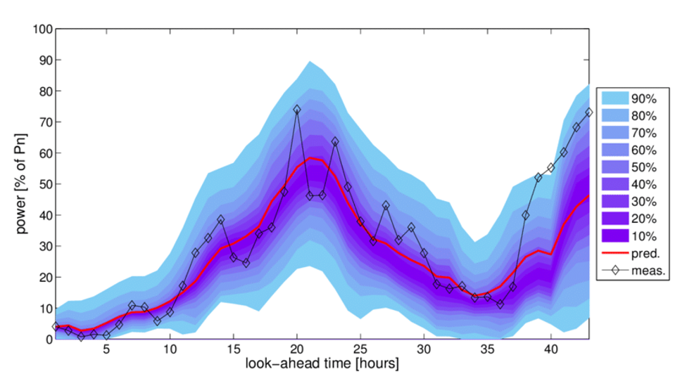
**Figure 13:** Probabilistic Forecasting Results of Wind Power With Prediction Intervals at Different Confidence Levels

Further analysis reveals that in low-power and stable weather-related intervals (such as the early stage and around 30 hours), the prediction interval width is appropriately increased, reflecting the model’s effective characterization of low-wind-speed nonlinear amplification and error uncertainty. In the medium-to-high-power interval, the prediction band converges faster, indicating that the model can provide more accurate predictions under relatively stable operating conditions. This “dynamic contraction-expansion” interval characteristic directly reflects the error state-based modeling and distribution inference mechanism proposed in this paper. Furthermore, the predicted mean curve closely approximates the actual observed values without significant systematic shifts, indicating that the wind speed correction (WSC) and state division mechanisms play a crucial role in reducing bias.

Figure 14 illustrates the data distribution characteristics of wind turbines in the three-dimensional space of wind speed, pitch angle, and output power, along with the processing results. The left figure shows the original data distribution, where green dots represent normal operating data and blue dots represent abnormal data. It can be observed that there are a large number of discrete points in the low wind speed and abnormal pitch angle regions. These abnormal samples deviate significantly from the typical power curve distribution, reflecting measurement errors, abnormal turbine control, or atypical operating states under stable weather conditions. The right figure shows the results after processing using the method presented in this paper, where red dots represent detected noise data, green dots represent retained normal samples, and orange dots represent clustering results used for further modeling. It can be seen that after data cleaning and state segmentation, the data distribution is more concentrated near the physically reasonable power curve, and different operating states are effectively distinguished.

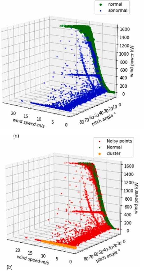
**Figure 14:** 3D Distribution of Wind Turbine Data Before and After Preprocessing

Figure 15 illustrates two typical forms of wind power prediction errors, phase error and amplitude error and compares their performance over time. The left figure shows that when the predicted curve shifts in time, even if the overall trend is similar to the actual curve, a large phase error will occur, with a corresponding MAE of 36.5%, indicating that time misalignment is one of the important sources of prediction deviation. The right figure shows the impact of amplitude error. Even when the predicted curve is aligned with the actual curve in time, the MAE is still about 20.7% due to the amplitude deviation, indicating that inaccurate power amplitude estimation can also significantly affect prediction performance. Combining the aforementioned mechanism analysis, it can be found that wind speed changes slowly but has strong uncertainty under stable weather conditions, making the prediction model more prone to lag or advance in time, thus causing phase error. At the same time, since wind speed is in the nonlinear sensitive range of the power curve, small wind speed deviations will be amplified into significant power amplitude errors. These two types of errors together constitute the main sources of wind power prediction errors, which are highly consistent with the “nonlinear amplification mechanism” and “error source decomposition model” proposed in §III-B.

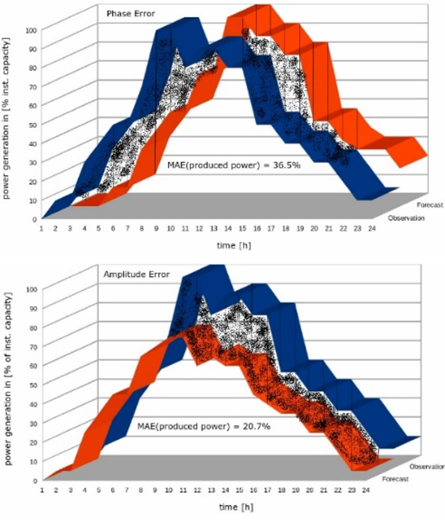
**Figure 15:** The Phase Error and Amplitude Error in Wind Power Forecasting

Figure 16 shows the frequency distribution of wind turbine operating states at different time scales, where blue (U), red (N), and green (S) represent different operating state categories (such as unstable/abnormal state, normal operation state, and low power or statically stable state). From the overall distribution, there are significant differences in the operating modes corresponding to different subfigures, reflecting the non-stationary nature of the wind power system over time. Specifically, in some periods (as shown in the early part of Figure 16(d), the green state has a significantly higher proportion, indicating that the turbines are in a long-term low-wind-speed or stable boundary layer-dominated operating state, consistent with the characteristics of low wind speed and weak fluctuations under statically stable weather conditions. In the middle and later stages, the proportions of red and blue states gradually increase, indicating that the wind field gradually enters a state of increased fluctuation or transition. Further analysis reveals that the state distribution exhibits a clear temporal evolution pattern within a daily cycle. For example, in some subfigures, the low-power state (S) has a higher proportion at night or in the early morning, while gradually decreasing during the day, which is consistent with the physical mechanism of surface radiative cooling leading to the formation of a stable boundary layer at night.

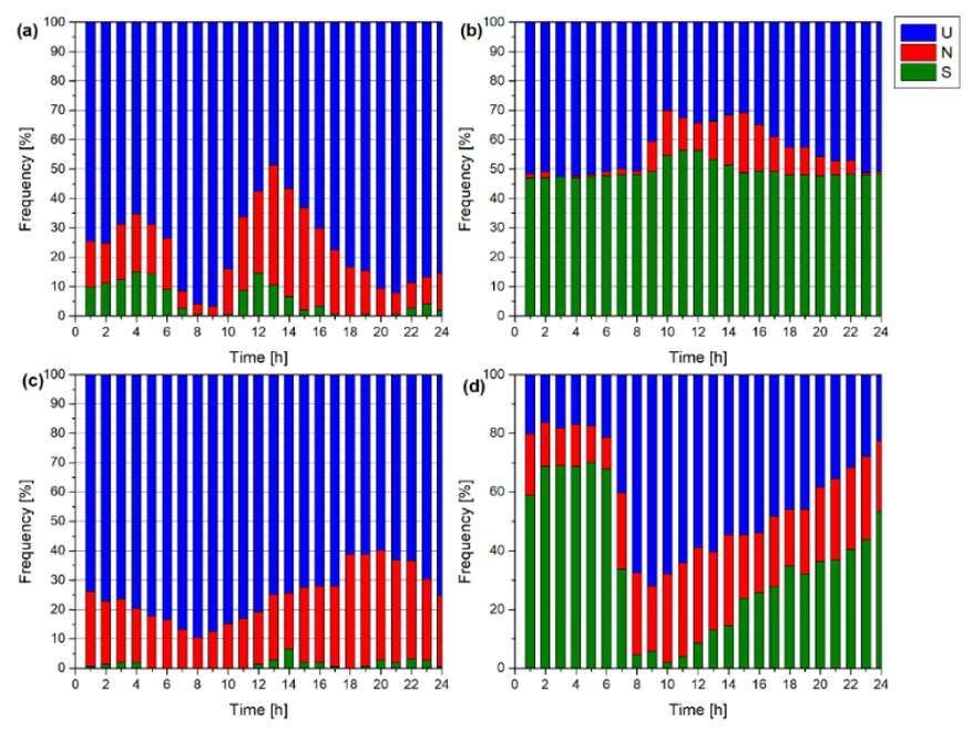
**Figure 16:** Temporal Distribution of Wind Turbine Operating States

Figure 17 analyzes the power output differences between the front and rear rows of wind turbines under different operating conditions and their relationship with the power coefficient \(c_{p}\) from multiple dimensions. Figures 17(a) and 17(b) show typical intraday variation characteristics. It can be observed that the overall output of the front row turbines is slightly higher than that of the rear row turbines, and the difference is more obvious during periods of higher wind speed. This reflects the suppressive effect of the wake effect on the downstream turbines. At the same time, the power coefficient decreases significantly during the daytime and rebounds at night or in the early morning, which is closely related to the changes in boundary layer stability. Figures 17(c) and 17(d) further show the trend of power change with turbulence intensity (TI). It can be seen that as TI increases, the overall turbine output decreases, while the difference between the front and rear rows gradually weakens, indicating that enhanced turbulence can weaken the wake effect to a certain extent. Figures 17(e) and 17(f) analyze power changes from the perspective of stability parameter (\(\zeta\)). It can be found that under stable stratification (\(\zeta\)\(\mathrm{>}\)0) conditions, the power of the rear units decreases more significantly, while under unstable conditions (\(\zeta\)\(\mathrm{<}\)0), the difference between the front and rear units decreases. This further verifies the mechanism by which the wake effect is amplified under stable weather conditions.

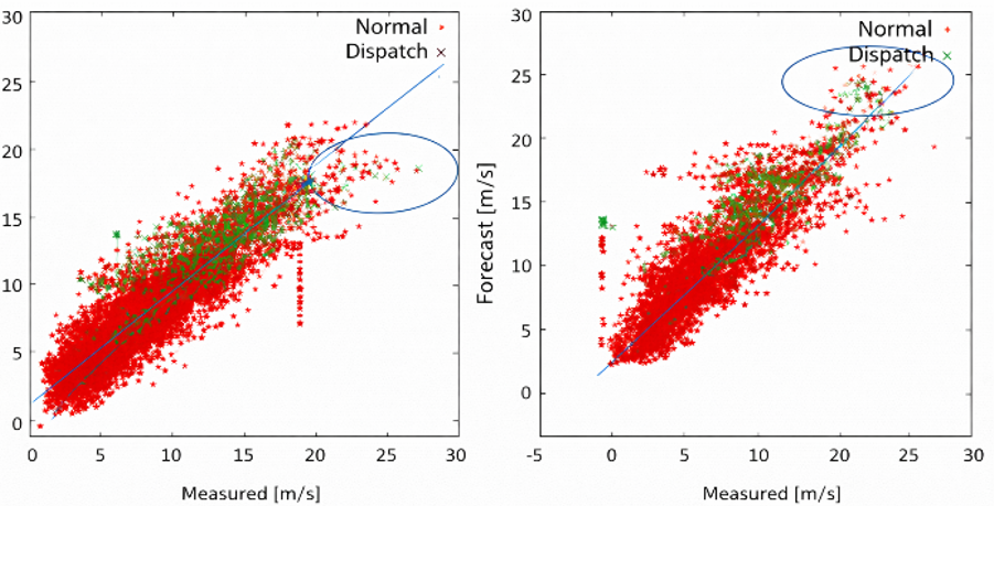
Figure 18 shows the scatterplot distribution between predicted and measured wind speeds, distinguishing between normal operation data and dispatch-related data. Overall, the predicted and measured values exhibit a relatively clear linear correlation, but significant deviations occur in the high-wind-speed range (above approximately 15 m/s), indicated by the blue elliptical areas. It can be observed that in these regions, predicted wind speeds are generally lower or higher than actual values, reflecting a systematic bias in numerical weather prediction under extreme or complex weather conditions. Simultaneously, dispatch data (green dots) exhibits different distribution characteristics from normal data in some intervals, indicating that wind power dispatch behavior indirectly affects the mapping relationship between wind speed and power. This phenomenon is consistent with the aforementioned analysis: under stable weather conditions or complex terrain, due to enhanced atmospheric stability and local flow field inhomogeneity, wind speed prediction errors exhibit significant structural biases, especially in the medium-to-high wind-speed range. This bias, on the one hand, is transformed into a larger power prediction error through the nonlinear amplification mechanism of the power curve; on the other hand, it also affects the model’s generalization ability under different operating conditions. Therefore, this paper introduces a wind speed correction module (WSC) to correct the NWP output, and combines state partitioning and error modeling mechanisms to address the deviations in different wind speed ranges, thereby effectively alleviating the above problems.

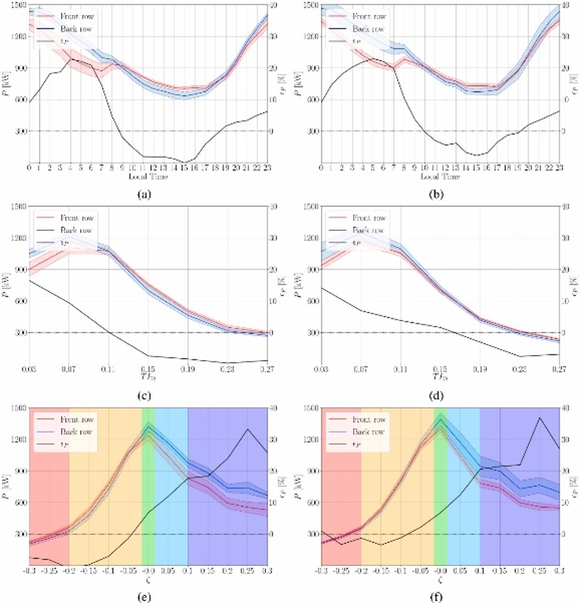
**Figure 17:** Impact of Wake Effects and Atmospheric Stability on Wind Turbine Power Output

Figure 19 statistically analyzes the characteristics of wind power distribution from three dimensions: atmospheric stability (stability class), turbulence intensity (\(TI_{78}\)) and turbine operating angle (e.g.,\(\theta _{76}\)). Figures 19(a) and 19(b) show the changes in power distribution under different stability classes and turbulence intensity ranges, respectively. It can be observed that under stable and very stable conditions, the overall power value is lower and the distribution is more concentrated, while the corresponding wind speed range is narrower, indicating that wind turbine operation is more easily limited by low energy input under calm and stable weather conditions. Under unstable or weakly stable conditions, the power distribution is more dispersed and the peak value is higher, reflecting that strong turbulent mixing can improve wind energy harvesting efficiency.

**Figure 18:** Scatter Plots of Forecasted Versus Measured Wind Speed

Furthermore, Figures 19(c) and 19(d) show the data duration distribution under different combinations of stability and turbulence intensity. It can be observed that the neutral and weakly stable states correspond to the largest amount of data, while the data under strongly stable and extreme turbulence conditions are relatively less, but they have a significant impact on the overall error distribution. This uneven distribution further illustrates that in actual modeling, different states must be modeled separately; otherwise, the model’s performance may degrade under low-frequency but high-impact statically stable weather scenarios.

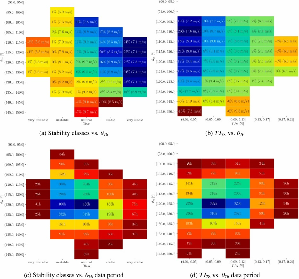
**Figure 19:** Joint Distribution of Wind Power With Atmospheric Stability Classes and Turbulence Intensity

Figure 20 further analyzes the influence of atmospheric stability classes and turbulence intensity \(TI_{78}\) on wind speed distribution from a temporal perspective, and compares the effects under different wind farms (CF1 and MO).

**Figure 20:** Joint Distributions of Atmospheric Stability Classes and Turbulence Intensity With Respect to Time of Day at Different Wind Farms (CF1 and MO)

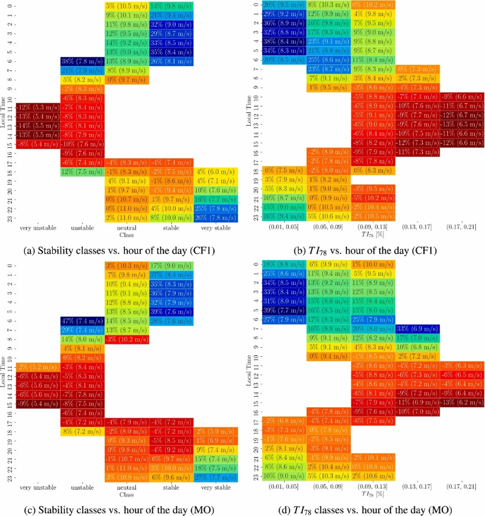
Figures 20(a) and 20(c) show the correspondence between stability classes and different times of day. It can be observed that during the night and early morning hours (approximately 0–6 am), the proportion of stable and strongly stable states is relatively high, corresponding to relatively low and less fluctuating wind speeds. This is consistent with the mechanism of surface radiative cooling leading to the formation of a stable boundary layer under stable weather conditions. During the daytime, especially from noon to afternoon, the proportion of neutral and unstable states increases, and the overall wind speed increases, reflecting enhanced turbulent mixing. Figures 20(b) and 20(d) further show the joint distribution characteristics of turbulence intensity over time. It can be found that the low turbulence intensity range is mainly concentrated in the stable nighttime period, while the high turbulence intensity mostly occurs in the unstable daytime period. At the same time, there are significant differences in the wind speed range corresponding to different turbulence ranges. A comparison of the CF1 and MO wind farms reveals that while the overall trend is consistent, the specific distributions differ, indicating that topography and local meteorological conditions modulate stability and turbulent structure. This coupling relationship between stability, turbulence, and time directly affects wind speed distribution and its prediction error characteristics. Particularly under stable weather conditions, where a stable boundary layer dominates, wind speed changes are more gradual but uncertainties increase, leading to significant state dependence and temporal clustering in prediction errors.

V. Conclusion

This paper addresses the problem of amplified wind power prediction errors under stable weather conditions by proposing a multi-module modeling framework that integrates mechanistic understanding and data-driven approaches. State partitioning mitigates non-stationarity, wind speed correction (WSC) reduces input error, and Markov chains (MC) characterize the temporal evolution of errors. Based on this, deep learning is combined to achieve deterministic prediction and probabilistic interval inference. Experimental results show that the proposed method outperforms mainstream models in both single-step and multi-step predictions, achieving higher coverage and more compact intervals in probabilistic predictions, particularly demonstrating stronger robustness under stable weather conditions. Ablation experiments further validate the effectiveness of each module. Overall, the proposed method effectively characterizes non-Gaussian uncertainty and improves prediction performance, providing reliable support for wind power dispatch and risk management. Future research could further enhance the model’s adaptability by combining online learning and high-resolution meteorological data.

Funding

This work was supported by the Science and Technology Project of State Grid Xinjiang Electric Power Co., Ltd. (No. 5230HQ25000C); the National Key Research and Development Program of China (2024YFB4204805).

Author Contributions

All authors contributed to the conception and design of the study, methodological development, data analysis, interpretation of the results, and preparation of the manuscript. All authors reviewed and approved the final version of the manuscript and agreed to be accountable for the integrity of the work.

Data Availability

The data supporting the findings of this study are available from the corresponding author upon reasonable request. Access to operational wind farm and SCADA data may be subject to institutional, commercial, and confidentiality restrictions.

Conflicts of Interest

The authors declare that they have no conflicts of interest related to this work.

Declaration of Generative AI and AI-Assisted Technologies

Generative artificial intelligence tools were used solely to assist with language editing and the preparation of LaTeX code. The authors reviewed and verified the accuracy, integrity, scientific content, and final wording of the manuscript and accept full responsibility for the published work.

References

[1] Li, Y., Liu, D., Wang, D., Xu, S., Ma, B., Yu, Y., … & Li, Y. (2025). Weather regimes of extreme wind speed events in Xinjiang: a 10–30 year return period analysis. Atmosphere, 16(10), 1117.
[2] Sun, X., Yang, T., Hu, Y., Zhang, H., Wang, J., Lu, W., … & Zha, J. (2025). Estimation and projection of development potential and stability for wind energy in Yunnan Province, China. Meteorology and Atmospheric Physics, 137(5), 44.
[3] Zhao, X., Huang, G., Lu, C., Li, Y., & Ren, J. (2024). Ensemble Bayesian model averaging projections of wind‐speed extremes for wind energy applications over China under climate change. Journal of Geophysical Research: Atmospheres, 129(1), e2023JD038806.
[4] Zhang, Q., Li, G., Chen, X., Yang, A., & Zhu, K. (2025). Enhancing renewable energy integration via robust multi-energy dispatch: a wind–PV–Hydrogen storage case study with spatiotemporal uncertainty quantification. Energies, 18(17), 4498.
[5] Lydia, M., Edwin Prem Kumar, G., & Akash, R. (2025). Wind speed and wind power forecasting models. Energy & Environment, 36(8), 3677-3713.
[6] Wang, L., Li, H., Zhu, Z., Xu, M., Liu, D., Baluch, S. M., & Zhao, Y. (2025). Nonlinear dynamics of ecosystem productivity and its driving mechanisms in arid regions: a case study of ebinur lake basin. Journal of Environmental Management, 386, 125770.
[7] Tang, J., Xiao, X., Han, M., Shan, R., Gu, D., Hu, T., … & Lu, J. (2024). China’s sustainable energy transition path to low-carbon renewable infrastructure manufacturing under green trade barriers. Sustainability, 16(8), 3387.
[8] Qin, Y., Zhou, M., Hao, Y., Huang, X., Tong, D., Huang, L., … & Zhu, T. (2024). Amplified positive effects on air quality, health, and renewable energy under China’s carbon neutral target. Nature Geoscience, 17(5), 411-418.
[9] Wang, X., Dai, C., Liu, G., Yang, X., Jing, J., & Ru, Q. (2025). Runoff prediction in the songhua river basin based on wep model. Hydrology, 12(10), 266.
[10] Liu, W., Ling, X., Li, C., & He, B. (2026). Optimizing CO2 concentrations and emissions based on the WRF-Chem model integrated with the 3DVAR and EAKF methods. Remote Sensing, 18(1), 174.
[11] Yang, B., Jin, A., Cheng, J., Zhou, S., & Jiang, B. (2025). Numerical simulation of ice crystal accretion and aerodynamic impacts on wind turbine blades in cold climates. Coatings, 15(2), 126.
[12] Jin, J., Li, L., Ben, W., Li, C., Liu, T., & Zheng, J. (2026). Exploring the necessity of low-carbon transition of power dispatching: a perspective of environmental efficiency assessment. Environment, Development and Sustainability, 1-25.
[13] Cai, W., Zhang, C., Zhang, S., Bai, Y., Callaghan, M., Chang, N., … & Gong, P. (2024). The 2024 China report of the Lancet Countdown on health and climate change: launching a new low-carbon, healthy journey. The Lancet Public Health, 9(12), e1070-e1088.
[14] Dong, X., Cao, Z., Guo, Y., Lin, J., Yan, H., Li, M., & Yao, P. (2024). Assessment of carbon storage in a multifunctional landscape: a case study of Central Asia. Land, 13(6), 801.
[15] Wang, Z., Shao, Z., Chen, R., Zhao, M., Jia, Z., Ma, Y., … & Zhang, B. (2025). NRBO-XGBoost-Optimized high-fidelity temperature correction for UAV-based TIR imagery and its application for monitoring coal fire. Fire, 8(12), 462.
[16] Wu, C., Wang, R., Lu, S., Tian, J., Yin, L., Wang, L., & Zheng, W. (2025). Time-series data-driven PM2. 5 forecasting: from theoretical framework to empirical analysis. Atmosphere, 16(3), 292.
[17] Luo, X., Zhang, C., & Bai, L. (2023). A fixed clustering protocol based on random relay strategy for EHWSN. Digital Communications and Networks, 9(1), 90-100.
[18] Liang, X., Cheng, W., Zhang, C., Wang, L., Yan, X., & Chen, Q. (2023). YOLOD: A task decoupled network based on YOLOv5. IEEE Transactions on Consumer Electronics, 69(4), 775-785.
[19] Zhang, C., Roh, B. H., & Shan, G. (2023, December). Poster: dynamic clustered federated framework for multi-domain network anomaly detection. In CoNEXT (Short Papers) (pp. 71-72).
[20] Liu, J., & Li, M. (2025). Characteristics and driving mechanisms of heatwaves in China during July and August. Atmosphere, 16(4), 434.
[21] Lu, H., & Hunt, A. (2025). Impact of climate policy uncertainty on regional new quality productive forces in China. Urban Science, 9(6), 189.
[22] Liu, X., Wen, W., Ma, X., Qian, D., Zhang, W., & Wang, S. (2025). Air pollution in a northwest Chinese valley city (2020–2024): Integrated WRF-HYSPLIT modeling of pollution characteristics, meteorological drivers, and transport pathways in Yining. Toxics, 13(10), 868.
[23] Zhang, W., Tan, N., & Ma, T. (2025). Mechanisms for the low-carbon transition of public transport energy systems: decoupling emissions and energy consumption in inner mongolia and the path to three-chain synergy. Energies, 18(18), 4817.
[24] Yang, M., Wei, Z., Long, J., Chen, L., Yu, H., Zeng, C., … & Wen, J. (2026). Application research on surveillance and predictive modeling of respiratory diseases in Baise City based on meteorological big data analysis. International Journal of Biometeorology, 70(3), 77.
[25] Wang, Z., Zhang, H., Wang, B., & Ding, Y. (2025). Towards a synergistic future: the impact of power sector decarbonization on sustainable development goals in China. Sustainable Production and Consumption, 56, 385-395.
[26] Muthuvel, D., & Qin, X. (2025). Probabilistic analysis of future drought propagation, persistence, and spatial concurrence in monsoon-dominant Asian regions under climate change. Hydrology and Earth System Sciences, 29(14), 3203-3225.