
An image channel can change substantially in numerical amplitude without changing the locations of its edges or the arrangement of its texture. A scalar gain and a spatially uniform offset provide a tractable description of this distinction: they alter intensity while preserving the sampling grid and, for positive gains, intensity ordering. A channel weight intended to describe organization within that grid may therefore benefit from independence of these two quantities. Such independence nevertheless raises a separate question. Removing sensitivity to intensity does not establish that the remaining descriptor identifies spatial organization. The distinction is consequential whenever a compressed statistic determines how strongly a complete feature map is transmitted.
Image translation makes this distinction concrete because the appearance of an output may vary while selected properties of its input remain recognizable. MUNIT represents images through a shared content code and a domain-specific style code, then combines content with different style values to obtain multiple outputs [1]. This representation separates factors at the level of a learned generator. It does not require every scalar summary used inside that generator to recover content. The information retained by an individual channel descriptor must therefore be assessed at the level of its own mathematical definition.
DRIT likewise separates content and attribute representations and introduces cross-cycle consistency for translation from unpaired images [2]. StarGAN v2 addresses diverse synthesis across multiple domains through learned style representations [3]. FUNIT changes the supervision available at inference by describing previously unseen target classes using only a few example images [4]. These approaches assign different roles to content, style, and class information. Their common relevance here is the need to distinguish changes that a representation should tolerate from differences that it should preserve. A scalar invariant can address the former requirement while remaining insufficient for the latter.
Spatial correspondence is treated more directly by contrastive unpaired translation. CUT encourages corresponding patches of the input and output to remain close in a learned feature space, using other patches as contrasting examples [5]. Its patchwise construction emphasizes that arrangement is an explicit part of some translation objectives. A channel statistic with no record of adjacency cannot, by itself, enforce such correspondence. This observation motivates an operator-level analysis that separates spectral concentration from the information needed to match neighboring image locations.
Diffusion-based translation places structure preservation within a conditional generation procedure. BBDM connects image domains through a Brownian bridge [6], while I\(^2\)SB learns diffusion bridges between boundary distributions for restoration [7]. These methods motivate distinguishing an internal descriptor’s algebraic properties from the independently evaluated quality of its generator’s outputs.
Channel attention supplies several instructive examples of this separation. Squeeze-and-excitation recalibrates feature channels through learned transformations of pooled channel descriptions [8]. ECA retains local cross-channel interactions while avoiding dimensionality reduction in the channel transformation [9]. In both cases, the pooling operation and the subsequent interaction between channels play distinct roles. Replacing a channel description changes only one of those roles. Consequently, a deterministic comparison with the global channel mean should not be interpreted as a comparison with an entire trained attention module.
CBAM applies channel and spatial attention sequentially [10]. A limitation of a scalar channel summary need not characterize that separate spatial stage. Differently arranged maps may receive equal weights while another network component distinguishes their locations. The present analysis therefore identifies the information available from the scalar itself.
Frequency-based channel attention introduces another distinction that is essential to the present analysis. FcaNet interprets channel compression using the discrete cosine transform and relates global average pooling to its lowest frequency component [11]. Fourier-domain pooling similarly controls dimensionality through truncation of a frequency representation [12]. Singular values describe a different object: the distribution of matrix energy among orthogonal left and right directions. They are not indexed by spatial frequency. An alternating separable pattern can have rank one, while a visually smooth map can require several singular components. Spectral concentration must accordingly be interpreted without equating it to smoothness or to the absence of rapid oscillation.
Second-order representations provide a useful context for this interpretation. Bilinear convolutional representations pool outer products to capture feature interactions in an orderless description [13]. GSoP uses covariance-based aggregation within convolutional networks to incorporate information beyond first-order pooling [14]. These constructions demonstrate why relationships among features can be more informative than their means alone. They also make the aggregation axes consequential. The row Gram matrix of one globally centered image channel describes interactions among its rows; it is not the cross-channel covariance of an arbitrary feature tensor, and a scalar trace ratio retains less information than either full matrix.
Style-related statistics illustrate why discarding mean intensity requires a specific purpose. SRM derives channel recalibration weights from pooled style information [15]. Adaptive instance normalization aligns channel means and variances between content and style features [16]. In those settings, quantities associated with appearance are used deliberately. The present question instead asks what remains when a descriptor is required to ignore a uniform offset and a nonzero scalar gain. Such invariance is a design constraint for the analysis, not a general assertion that illumination or contrast is irrelevant to image translation.
Group normalization computes statistics across selected channels and spatial positions independently of batch size [17]. Here, one global mean is subtracted from each two-dimensional channel. This operation neither centers individual rows nor generally reduces rank below the spatial dimension. Spectral bounds must respect that specific centering operation.
Non-identifiability is also relevant to the interpretation of texture. Correlations of convolutional responses support texture synthesis without specifying a unique arrangement of image pixels [18]. Separately, evidence of texture bias in particular ImageNet-trained convolutional networks shows that texture sensitivity and shape sensitivity need not coincide [19]. Neither result proves the behavior of the operator examined here. They motivate a more precise question about it: whether equal concentration can coexist with substantially different local variation. That question can be answered constructively, without assigning semantic labels to generated matrices.
The descriptor studied below is the normalized second spectral moment of the Gram matrix of a globally centered channel. Equivalently, it is the sum of squared proportions of the centered singular-value energy. Normalized trace concentration has an established connection with covariance sphericity [20]; the underlying statistic is not introduced here as a new measure of dimensionality. Its bounded affine transformation supplies a scalar gate, and its reciprocal gives a participation-ratio dimensionality. The analysis concerns the consequences of applying this construction to centered channel matrices, including its invariance, information loss, and behavior near zero centered energy.
The research question is whether this gate can be invariant to affine intensity changes while still distinguishing changes in spatial arrangement. The answer requires examining the scalar weight and the weighted map separately. Multiplication by a spatially uniform positive weight retains the arrangement already present in a map, even when the weight cannot identify that arrangement. Independent row and column permutations provide an exact test: they preserve singular values while potentially changing nearly every adjacency relation. Their effect on discrete neighboring-pixel differences can therefore expose information that the scalar does not encode.
The investigation combines algebraic results with computations on 384 explicitly generated \(32\times32\) matrices from six families and a separate diagnostic using two credited photographs. The generated collection contains smooth blobs, horizontal oscillations, diagonal edges, checker textures, Gaussian noise, and power-law spectra. Its diversity is chosen to separate concentration from familiar visual categories, rather than to represent an image population. Affine transformations, controlled additive perturbations, spatial permutations, and decreasing-contrast inputs interrogate different properties of the same gate. The computations retain their defining arrays and parameters, allowing the numerical statements to be checked without network training or undisclosed image acquisition.
Exact gain and offset invariance holds for nonconstant matrices, whereas the permutation construction defeats spatial identification from the scalar. A relative perturbation bound applies away from zero centered energy. Constant inputs require separate treatment because different directions of vanishing contrast give different gate limits. These distinct conditions determine the descriptor’s invariance, spatial ambiguity, and numerical boundary.
The motivating data is the retained-length comparison, its five retained lengths and paired FID and energy-of-gradient values are in Table 1 [21]. Only that parameter comparison used in the present manuscript. Its printed task label is Cezanne2photo, although the adjacent discussion describes seasonal imagery.
| Retained length \(N\) | FID | Energy of gradient |
|---|---|---|
| 16 | 77.15 | 1001.83 |
| 32 | 74.64 | 972.50 |
| 64 | 62.19 | 1024.77 |
| 128 | 57.36 | 1197.49 |
| 256 | 71.59 | 1007.10 |
The smallest listed FID occurs at 128 rather than at either endpoint. That ordering supports a narrowly defined observation about five settings. It supplies neither a distribution of preferred ranks nor uncertainty about their performance. The present unit of analysis is instead a real square matrix representing one channel. Its gate is calculated independently of a discriminator, style encoder, or supervised target. This choice allows the transformation law to be tested directly and prevents image-level generation scores from being used as evidence for an unmeasured intermediate mechanism.
Six families supply different arrangements of smoothness, periodicity, edges, and broadband variation. Each family contains 64 realizations on a \(32\times32\) grid, yielding 384 matrices. Coordinates are \(x_j=-1+2j/32\) and \(y_i=-1+2i/32\), with indices from zero to 31. Family index \(f\in\{0,\ldots,5\}\) and realization index \(r\in\{0,\ldots,63\}\) determine the NumPy random-generator seed \(20250908+10000f+r\). Every realized parameter is retained in a machine-readable manifest. NumPy supplies the array operations and pseudorandom draws [22].
The smooth family is a separable Gaussian profile with center coordinates independently uniform on \([-0.45,0.45]\) and widths independently uniform on \([0.18,0.50]\). Its raw matrix has rank one; removal of a nonzero global mean can increase that rank to two. The horizontal family combines two separable oscillations with integer \(k\) uniform on \(\{2,\ldots,6\}\), phases \(\phi,\psi\) uniform on \([0,2\pi]\), and mixing amplitude \(\eta\) uniform on \([0.10,0.40]\). Their definitions are
The finite grid contains whole oscillation periods in the vertical direction. Thus the bands have zero mean in exact arithmetic and at most two nonzero singular values. Their relatively small algebraic rank is deliberate: it prevents a high-frequency visual appearance from being equated with a diffuse singular spectrum.
The edge family uses \(R_{ij}=\tanh[(x_j\cos\theta+y_i\sin\theta-d)/w]\), where \(\theta\) is uniform on \([\pi/6,\pi/3]\), displacement \(d\) on \([-0.35,0.35]\), and width \(w\) on \([0.04,0.18]\). Checker textures combine two separable products,
where \(k_x,k_y\) are independent integers from two through seven, the phases are independently uniform on \([0,2\pi]\), and \(\eta\) is uniform on \([0.15,0.55]\). Distinct sampled frequencies make the two separable components orthogonal along each axis. The resulting concentration can therefore be checked against \((1+\eta^4)/(1+\eta^2)^2\).
Gaussian matrices contain independent standard normal entries. The sixth family filters an independent Gaussian array in the discrete Fourier domain with amplitude \((1+k^2+l^2)^{-\beta/4}\), where signed frequencies follow the discrete Fourier convention and \(\beta\) is uniform on \([1,3]\). Taking the real inverse transform yields a radially filtered array. The squared filter amplitude approaches a radial power law away from zero frequency; no exact slope is asserted for each finite realization. These six generating rules define computational signals rather than categories sampled from a natural-image population.
Each raw matrix \(R\) is standardized as
where \(J\) is the all-ones matrix. Every numerical input consequently has approximately zero global mean and unit root mean square. Both raw and standardized arrays are retained. Standardization fixes a common intensity scale for the disturbance experiments without making the matrices statistically interchangeable. There are no training, validation, or test partitions because no parameters are fitted and no predictive model is selected.
Two photographs distributed through SciPy [23] provide a separate check on recognizable spatial content. The raccoon image is credited to Judy Weggelaar and the ascent image to Steve Hillebrand, USFWS; their distribution pages identify CC0. The project records the corresponding photograph URLs and byte-level array hashes. The raccoon array has dimensions \(768\times1024\times3\). Columns 128 through 895 are retained, RGB values are divided by 255 and combined with weights \((0.2126,0.7152,0.0722)\), and nonoverlapping \(6\times6\) block averages produce a \(128\times128\) array. These weights define an encoded-value grayscale conversion, not a physical luminance measurement. The \(512\times512\) ascent array is divided by 255 and reduced using \(4\times4\) block averages.
Each processed photograph is partitioned into sixteen nonoverlapping \(32\times32\) patches. The resulting 32 patches are a finite diagnostic collection with strong within-photograph dependence. They are not treated as independent natural scenes. The complete \(128\times128\) images are also evaluated to relate exact spectral invariance to recognizable adjacency. All processing is deterministic and uses no learned image synthesis. Permuted images represent explicitly reordered measurements of the same pixel arrays.
For a feature tensor with channels \(F_c\in\mathbb{R}^{n\times n}\), the operator acts independently on each channel. Suppressing \(c\) for clarity, define the orthogonal centering operation \(C(F)=F-\overline FJ\) and let \(Z=C(F)\). For nonzero \(Z\), squared singular-value proportions and concentration are
The bounded gate and weighted channel are
At \(Z=0\), the numerical convention is \(g(F)=1/2\). No spectral dimension is inferred at that point. Concentration is an established trace-ratio type of sphericity statistic [20]; the present contribution concerns its explicit gating interpretation and limitations. The participation quantity \(r_2=1/q\) differs from Shannon-entropy effective rank, including in the normalization of singular values [24]. Neither quantity is identical to algebraic rank for a general unequal spectrum.
The gate contains no fitted parameter, rank cutoff, or denominator regularizer. Its affine scaling assigns spectra with equal energy across all singular components a half-unit weight and rank-one spectra a unit weight. These endpoints are chosen to preserve a positive output multiplier, rather than calibrated from predictive labels. Favoring concentration is a design choice whose consequences are assessed, not a claim that every concentrated channel is useful. Unlike cross-channel covariance pooling, the Gram product here relates spatial rows within a single map. Established second-order representation methods provide context for using matrix summaries but are not implementations of this channelwise operator [25], [26].
In floating-point arithmetic, \(Z\) is divided first by its largest absolute entry and then by its Frobenius norm. If the first divisor is exactly zero, the constant branch is taken. Otherwise the resulting matrix \(U\) has unit Frobenius norm, and \(q=\left\lVert UU^\top\right\rVert_F^2\). A separate singular-value calculation of \(\sum_i\sigma_i(U)^4\) verifies this identity. The two normalizations reduce avoidable dynamic-range problems; they cannot recover differences already rounded away when \(F\) was formed. No clipping of transformed intensities is performed.
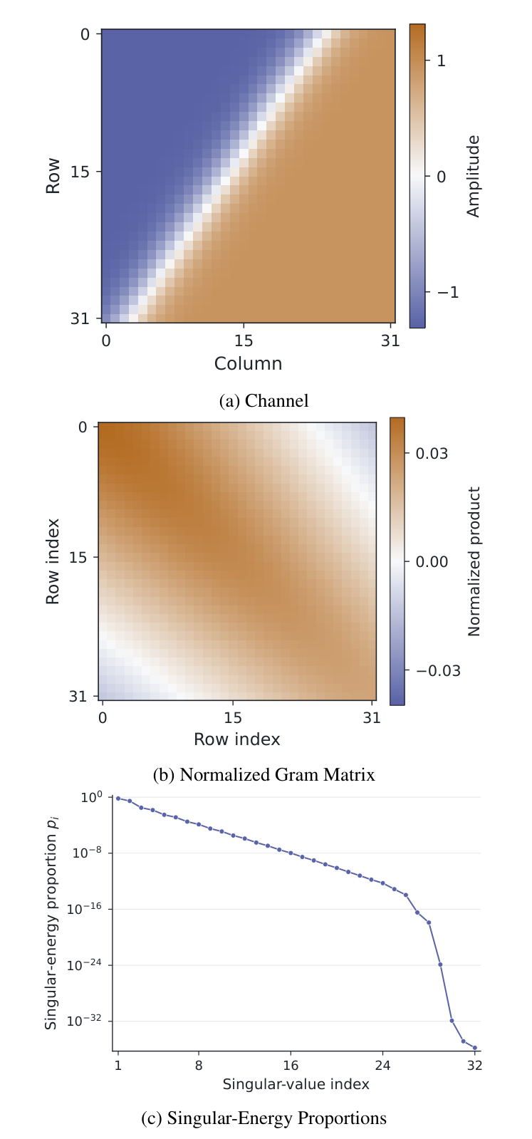
The numerical construction is displayed in Figure 1 for the first diagonal-edge realization. The channel image retains its oblique transition; the normalized row Gram matrix displays row interactions, and the singular-energy proportions describe their concentration. These are three calculations on one stored array, rather than architectural components of a trained network.
The plotted spectrum is strongly concentrated without being a single nonzero component. Its smallest displayed values are numerical outputs near the precision limit, not resolved physical measurements. The gate uses the complete summed concentration, so those tiny values do not justify an independently chosen retained-rank threshold.
The affine experiment crosses five gains, \(a\in\{0.25,0.5,1,2,4\}\), with five offsets, \(b\in\{-2,-0.5,0,0.5,2\}\), in \(aF+bJ\). This produces 9,600 generated-map cases, including 384 identity cases, and 800 photograph-patch cases. The uncentered comparison uses the same formula on \(F\) without subtracting its mean. Global average pooling is inspected only as a scalar descriptor; its raw numerical changes are not compared as if they were learned attention errors.
For additive disturbances, twenty Gaussian directions per generated matrix are centered and scaled to relative Frobenius norms \(\rho\in\{0,0.01,0.03,0.1,0.3,1\}\). The same direction is used at the six amplitudes for each matrix and repetition. Consequently the noise is a Gaussian direction conditioned to a specified norm, rather than a new unconditioned draw at every amplitude. This design produces 46,080 evaluations. Seeds and complete ordering are specified by the supplied program. Signed differences distinguish concentration loss from gain, while absolute differences quantify the size of the gate response.
Twenty independent row and column permutations per generated matrix yield 7,680 additional cases. Another twenty per photograph patch yield 640 cases. For nonconstant inputs, spatial variation is evaluated using
Internal neighbour pairs are counted once without periodic wrapping. This dimensionless difference energy measures adjacency variation, not perceptual quality. It is distinct from the differently normalized energy-of-gradient values in Table 1.
Finally, \(J+10^{-k}F\) is represented in double precision for \(k=0,\ldots,18\), giving 7,296 near-constant cases. The experiment records gate deviations and exact constant-branch counts. Directional derivatives are checked on all 384 generated matrices at three central-difference steps, providing 1,152 comparisons. All summaries describe the executed finite collections. Sample standard deviations summarize realization spread; they are not standard errors for a population. No significance testing, confidence interval, or inferred translation score is used. Matplotlib is used exclusively to render the retained numerical outputs [27].
The numerical specification distinguishes generation randomness from transformation randomness. Each disturbance direction uses seed \(20250909+1000m+r\), where \(m\) is the stored matrix index and \(r\) the repetition. Permutations use \(20250910+1000m+r\). Complete-photograph permutations use consecutive seeds 20250911 and 20250912; patch permutations use \(20250912+100m+r\). Derivative directions use \(20250913+m\) and are normalized to unit Frobenius norm before central differences are taken. The integer seeds identify deterministic pseudorandom constructions. They are not dates of image acquisition or evidence of prospective registration. Shared directions across disturbance amplitudes preserve a paired comparison and must remain shared when the calculations are repeated.
Each observation retains the matrix identity, generating family, transformation parameters, and repetition. Summaries can therefore be reconstructed from individual records. Both downloaded integer photographs and processed arrays are bundled, making the grayscale calculation and block averages independently checkable. Hashes establish array identity; the analytical identities and numerical comparisons separately assess correctness.
A dense square Gram product requires cubic arithmetic and quadratic storage, matching the leading scaling of a dense singular-value calculation. No timing advantage is claimed: practical costs depend on implementation, and the supplied verification routine computes both forms. The operator requires a separate product per channel and contains no learned cross-channel interaction. A surrounding architecture would need its own evaluation.
Proposition 1 (Range and participation). For \(n\ge2\) and \(C(F)\ne0\), \(1/n\le q(F)\le1\), \(1/2\le g(F)\le1\), and \(1\le r_2(F)\le\operatorname{rank}C(F)\). Equal nonzero singular values attain the participation upper bound.
Proof. The \(p_i\) in Eq. (3) are nonnegative and sum to one. Cauchy–Schwarz gives \(1\le n\sum_i p_i^2\), while \(p_i^2\le p_i\) gives \(\sum_i p_i^2\le1\). If exactly \(r\) proportions are positive, the same inequality over those entries gives \(q\ge1/r\). The affine definition of \(g\) preserves these bounds. Equality \(q=1/r\) requires equal positive proportions.
The distinction between algebraic rank and participation matters when many small singular values accompany a few large ones. Algebraic rank counts every nonzero value; participation weights the distribution continuously. Global mean removal imposes one scalar constraint, \(\boldsymbol{1}^{\top}Z\boldsymbol{1}=0\), and does not imply rank at most \(n-1\). Retaining \(1/n\) in the gate normalization is therefore necessary. A rank-one centered matrix has the maximum gate even if its nonzero entries oscillate rapidly across the grid.
Proposition 2 (Affine-intensity invariance). For any \(F\), real \(b\), and nonzero real \(a\), \(g(aF+bJ)=g(F)\). The weighted map obeys
Proof. Linearity of centering gives \(C(aF+bJ)=aC(F)\). The numerator and denominator in Eq. (3) both scale by \(a^4\), including for negative \(a\). Constant matrices remain constant and preserve the half-unit convention. Multiplying the transformed input by its unchanged gate gives Eq. (6).
The result concerns global affine intensities in real arithmetic. Saturation, quantization, spatially varying light, and nonlinear response are different operations. A zero gain collapses every input to a constant and is excluded from gate invariance. The weighted map is gain equivariant, but its offset response is modulated by \(g(F)\). It does not become illumination invariant merely because its multiplier does.
Proposition 3 (Permutation equivalence). For row and column permutation matrices \(P,Q\), \(g(PFQ^{\top})=g(F)\) and \(T(PFQ^{\top})=PT(F)Q^{\top}\). Moreover,
Proof. Permutations preserve the global mean and satisfy \(PJQ^{\top}=J\). Therefore \(C(PFQ^{\top})=PC(F)Q^{\top}\). Orthogonality of \(P,Q\) preserves the singular values. The gate is unchanged; multiplying by the permuted matrix establishes equivariance and Eq. (7).
Independent permutations can change which pixels are neighbours while preserving the entire singular spectrum. Consequently even the complete spectrum cannot determine spatial adjacency under this transformation class. A scalar concentration inherits that non-identifiability. Eq. (7) supplies an equally important qualification: the feature arrays remain different, and multiplication by a positive gate does not erase their difference. Arbitrary permutations of all pixels are not covered; such rearrangements need not preserve singular values.
Lemma 1 (Normalized matrices). For nonzero matrices \(X,Y\), let \(r=\left\lVert X\right\rVert_F\), \(s=\left\lVert Y\right\rVert_F\), \(A=X/r\), and \(B=Y/s\). Then \(\left\lVert A-B\right\rVert_F\le2\left\lVert X-Y\right\rVert_F/(r+s)\).
Proof. Writing \(d=\left\lVert A-B\right\rVert_F\le2\) gives \(\left\lVert X-Y\right\rVert_F^2=(r-s)^2+rsd^2\). Subtracting \((r+s)^2d^2\) from four times this identity leaves \((r-s)^2(4-d^2)\ge0\), which proves the bound.
The normalization estimate depends on the sum of endpoint Frobenius norms rather than an eigenvalue separation. It remains meaningful when singular values coincide, provided neither centered matrix is zero. It is thus suited to a scalar spectral moment, whose definition does not require choosing singular vectors.
Proposition 4 (Gate disturbance). For nonzero centered endpoints \(X\) and \(Y=X+E\),
Proof. Using the lemma, define \(M=AA^{\top}\) and \(N=BB^{\top}\). Their Frobenius norms are at most one. The factorization \(M-N=(A-B)A^{\top}+B(A-B)^{\top}\) gives \(\left\lVert M-N\right\rVert_F\le2\left\lVert A-B\right\rVert_F\). Consequently \(|q(X)-q(Y)|=|\langle M-N,M+N\rangle_F|\le4\left\lVert A-B\right\rVert_F\le8\left\lVert E\right\rVert_F/(\left\lVert X\right\rVert_F+\left\lVert Y\right\rVert_F)\). Eq. (4) and its half-unit range establish the result.
For an uncentered disturbance \(H\), use \(E=C(H)\); orthogonal projection ensures \(\left\lVert C(H)\right\rVert_F\le\left\lVert H\right\rVert_F\). The estimate is a conservative certificate rather than an optimal constant. Its denominator explains why a small absolute disturbance may be substantial relative to weak contrast. At large relative disturbances the half-unit range can dominate, leaving little additional information about actual sensitivity.
For nonzero \(Z\), set \(e=\left\lVert Z\right\rVert_F^2\). Ordinary matrix differentiation gives
Indeed, differentiating \(\operatorname{tr}[(ZZ^{\top})^2]\) gives \(4ZZ^{\top}Z\), and differentiating \(e\) gives \(2Z\). The centering operator is self-adjoint in the Frobenius inner product, yielding the second identity. This direct expression belongs to structured matrix differentiation [28]; it does not differentiate individual singular vectors. Coincident singular values therefore introduce no singular-vector denominator. Near-zero centered energy remains a separate conditioning problem.
Proposition 5 (No continuous gate extension at constants). No value assigned at a constant matrix can make \(g\) continuous there. With the stated convention, \(T\) is continuous at zero and discontinuous at every nonzero constant matrix.
Proof. Let \(H_1=e_1(e_1-e_2)^{\top}\) and \(H_2=\operatorname{diag}(1,-1,0,\ldots,0)\). Both are globally centered, with concentrations one and one half. For any nonzero \(t\), the matrices \(cJ+tH_1\) and \(cJ+tH_2\) therefore have different fixed gate values. As \(t\) tends to zero, both approach \(cJ\), so no single gate value supplies continuity. However, \(\left\lVert T(F)\right\rVert_F\le\left\lVert F\right\rVert_F\) proves continuity of \(T\) at zero. When \(c\ne0\), the rank-one path gives \(T(cJ+tH_1)\to cJ\), whereas \(T(cJ)=cJ/2\).
Exact gain invariance preserves direction-dependent spectral information at arbitrarily small contrast. The price is the absence of a continuous scalar limit when that contrast vanishes. This mathematical property must be distinguished from finite-precision rounding, which may replace a nearly constant array by an exactly constant one before evaluation. Both mechanisms matter, but they occur at different levels of the computation.
The derivative also clarifies which perturbation directions are invisible locally. Its Frobenius inner products with the all-ones matrix and with the centered input are zero. The first identity follows from the final centering operation; the second follows from homogeneity of the trace ratio. Thus infinitesimal offset and gain changes agree with the finite transformation law. Other directions can alter the concentration even when they preserve the global mean. This separation prevents exact affine invariance from being mistaken for insensitivity to all low-amplitude changes. The derivative remains a property of the stated real-valued map and does not describe gradients through intensity clipping or quantization.
For an objective depending on the weighted channel, differentiation includes both the direct input path and the gate’s input dependence. The checks here verify the descriptor derivative, not an optimizer trajectory. Avoiding singular-vector differentiation consequently does not establish convergence or stability of a trained network containing the operator.
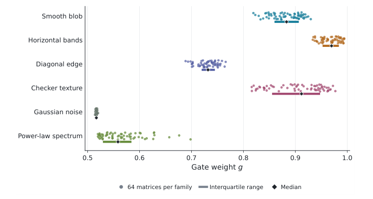
The generated collection spans substantially different participation values while keeping the intensity scale fixed. Table 2 gives family means and sample standard deviations for the gate, together with mean participation. Horizontal oscillations receive the largest average weight, 0.967640, and Gaussian noise the smallest, 0.516776. The observed concentration range is 0.058312–0.988881, corresponding to gate values 0.513967–0.994261. All values lie within the analytical interval. None of the standardized matrices enters the constant branch.
| Family | Mean \(q\) | Mean \(g\) | SD of \(g\) | Mean \(r_2\) |
|---|---|---|---|---|
| Smooth blob | 0.771672 | 0.882154 | 0.028641 | 1.302718 |
| Horizontal oscillation | 0.937302 | 0.967640 | 0.017886 | 1.068342 |
| Diagonal edge | 0.478520 | 0.730849 | 0.018480 | 2.101768 |
| Checker texture | 0.815191 | 0.904615 | 0.049984 | 1.244958 |
| Gaussian noise | 0.063754 | 0.516776 | 0.001137 | 15.703623 |
| Power-law spectrum | 0.157434 | 0.565127 | 0.040382 | 7.876089 |
The individual weights in Figure 2 make the within-family spread explicit. Each dot is one matrix; diamonds and thick segments mark medians and interquartile ranges. The narrow Gaussian distribution and the asymmetric power-law distribution are visible without treating either summary as a confidence interval.
The overlap between blob and checker weights shows that a coefficient can be similar for smooth and oscillatory patterns. Their separate construction therefore matters more than assigning a visual category to the coefficient alone.
The low mean participation of checker textures follows from their two orthogonal separable terms, even though the images contain many alternating cells. Smooth blobs have higher participation than their raw rank-one construction might suggest because global centering subtracts a second separable matrix. Diagonal edges distribute energy more broadly because the transition is oblique to the row and column axes. These relationships explain the numerical ordering in terms of the specified generating equations. They do not identify an ordering of visual usefulness. The dispersion of power-law results reflects the varying spectral exponent and realization, whereas the Gaussian family is tightly concentrated around a diffuse singular-energy distribution.
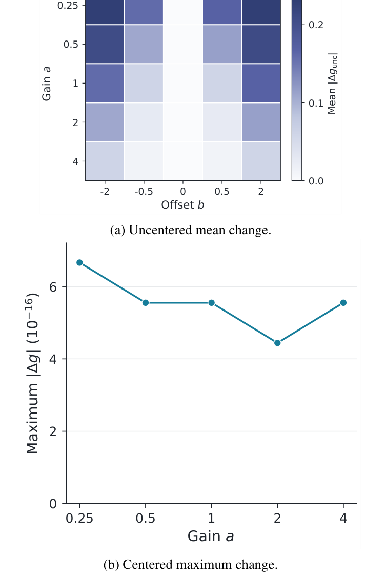
Across all 9,600 affine transformations, the centered gate changes by at most \(6.6613\times10^{-16}\), with mean absolute change \(3.3168\times10^{-17}\). The uncentered version changes by 0.091771 on average and by 0.471307 at its maximum. Because both use the same spectral-energy normalization, the offset sensitivity is attributable to retaining the mean component rather than to a difference in gate scaling. At zero offset, nonzero gains preserve either concentration in exact arithmetic. Nonzero offsets can instead add a dominant rank-one component to the uncentered matrix.
The gain–offset combinations are resolved in Figure 3. Each heatmap cell averages the uncentered change over 384 matrices, while the companion plot shows the largest centered change at each gain over all offsets and matrices.
The strongest uncentered changes occur when the offset dominates the scaled contrast. The centered curve remains on the roundoff scale; its small nonmonotonic variations are not evidence of a meaningful dependence on gain.
Global-average pooling changes by exactly the assigned offset in real arithmetic, giving mean and maximum absolute changes of 1.0 and 2.0 over this design. This response is expected for a mean descriptor and is not interpreted as an attention-performance ranking. For the 32 photograph patches, 800 affine cases produce a maximum centered-gate change of \(2.2204\times10^{-15}\). Their nonzero starting means provide a useful check beyond the standardized generated matrices, but the same algebra already predicts the outcome.
Independent singular-value calculations agree with the Gram expression within \(1.8874\times10^{-15}\) for centered cases and \(2.9976\times10^{-15}\) for uncentered cases. These are numerical discrepancies between equivalent formulas, not uncertainty in an empirical outcome. The directional derivative checks give maximum absolute errors of \(9.33\times10^{-12}\), \(4.38\times10^{-12}\), and \(4.32\times10^{-11}\) at steps \(10^{-3}\), \(10^{-4}\), and \(10^{-5}\). The smallest step does not give the smallest error because subtractive cancellation competes with truncation error. Agreement across these checks supports the implementation of the explicit operator.
The 46,080 disturbance cases give the absolute changes summarized in Table 3. At relative norm 0.01, the mean change is below \(10^{-4}\). At 0.1 it increases to 0.004869, with maximum 0.012615. Larger disturbances shift the gate further: at relative norm one, the mean absolute change is 0.183920 and the maximum 0.384523. Mean signed changes are negative at every nonzero amplitude, reaching \(-0.183770\) at the largest amplitude. The additive directions therefore generally spread energy across more singular components for this collection.
| \(\rho\) | Mean signed change | Mean absolute change | Maximum | Mean bound |
|---|---|---|---|---|
| 0.00 | 0.000000 | 0.000000 | 0.000000 | 0.000000 |
| 0.01 | -0.000049 | 0.000088 | 0.000586 | 0.020645 |
| 0.03 | -0.000440 | 0.000479 | 0.002148 | 0.061921 |
| 0.10 | -0.004829 | 0.004869 | 0.012615 | 0.205934 |
| 0.30 | -0.038817 | 0.038897 | 0.082632 | 0.500000 |
| 1.00 | -0.183770 | 0.183920 | 0.384523 | 0.500000 |
The bound is satisfied in every case within the \(10^{-12}\) verification tolerance. Its mean value at relative norm 0.1 is 0.205934, much larger than both the observed mean and maximum change. At 0.3 and one it is the half-unit range limit throughout. Thus the certificate establishes admissibility and explains the dependence on relative contrast, while providing a deliberately loose prediction of the sampled Gaussian directions. A lower gate under disturbance does not demonstrate removal of that disturbance from the weighted image.
The family responses in Figure 4 separate concentrated inputs from the already diffuse Gaussian family. Lines connect measured amplitude settings, and the dashed curve is the pooled mean of the deterministic bound. The zero-amplitude checks are omitted from the logarithmic axes.
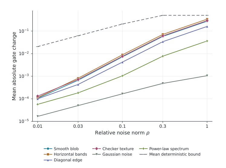
The separation of response curves grows with disturbance amplitude. Its interpretation concerns the starting singular-energy distribution, while the dashed curve certifies a permissible displacement rather than fitting the observed trajectories.
Family-specific changes reveal information hidden by the overall disturbance average. At relative norm 0.1, mean signed changes are approximately \(-0.00893\) for horizontal oscillations, \(-0.00763\) for checker textures, \(-0.00723\) for blobs, and \(-0.004225\) for diagonal edges. The Gaussian family instead has a mean close to zero and includes changes of either sign. Its singular energy is already spread across many directions, so another isotropically sampled direction does not systematically move it toward a substantially less concentrated state. Power-law matrices occupy an intermediate position, with mean signed change approximately \(-0.00097\) at the same amplitude.
These differences persist at the largest disturbance. Horizontal oscillations have mean signed change approximately \(-0.33871\), whereas the Gaussian mean remains approximately \(-0.00016\). The contrast does not rank the families by vulnerability to visual corruption: every disturbance is normalized relative to the matrix norm, and no perceptual target is defined. It instead describes how the same radial displacement acts on different starting spectra. A concentrated input has considerably more room to move downward within the gate interval than a diffuse input already close to its lower endpoint. That geometric constraint is necessary when interpreting averages across families.
The 7,680 row-and-column permutation cases preserve the scalar gate within \(6.6613\times10^{-16}\). Nevertheless mean normalized difference energy rises from 0.063130 to 2.564737 for blobs and from 0.038214 to 2.467749 for edges. Checker textures increase from 1.791883 to 3.982814. Gaussian noise instead changes little, from 3.882071 to 3.876588, consistent with the lack of preferred spatial ordering in its generating distribution. Mean relative input distance is 1.412224 across the collection. The corresponding relative weighted-output distance agrees within \(8.88\times10^{-16}\), as predicted by the common scalar multiplier.
The complete raccoon image has gate 0.586287 before and after its prescribed permutation, while its difference energy increases from 0.325416 to 3.228410. The ascent image has unchanged gate 0.553993 and an increase from 0.619059 to 3.532646. These are increases of approximately 9.92 and 5.71 times, respectively, calculated from the retained image arrays. Among the 640 patch permutations, the largest gate difference is \(3.33\times10^{-16}\). Recognizable image content is therefore compatible with exact descriptor collisions; the construction is not restricted to analytic textures.
The photographic pairs in Figure 5 display the actual processed arrays before and after row-and-column reordering. All panels retain the same grayscale limits; no translated image or reconstructed scene is substituted for the computed permutation.
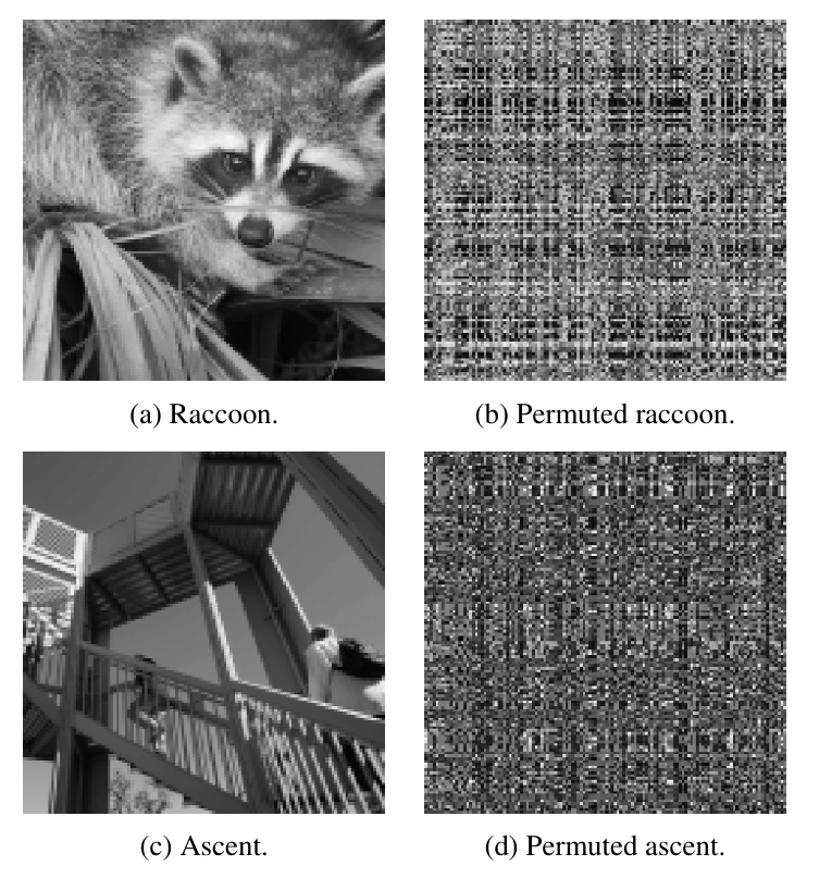
The recognizable contours are displaced despite exact equality within each pair. The visible changes are retained in the weighted arrays, so the equality identifies a limitation of the scalar description rather than disappearance of image information.
The complete set of generated-map permutations appears in Figure 6. Each point represents a stored pair, and the diagonal marks unchanged difference energy. Concentrated families lie predominantly above that line, while Gaussian realizations cluster near it.
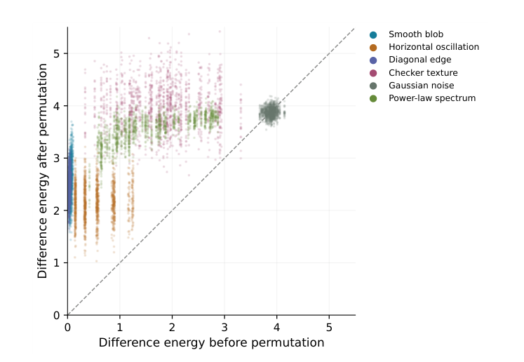
The nearly vertical groupings arise because each matrix has one pre-permutation energy and twenty reordered values. They are repeated transformations of specified inputs, not twenty newly acquired independent images.
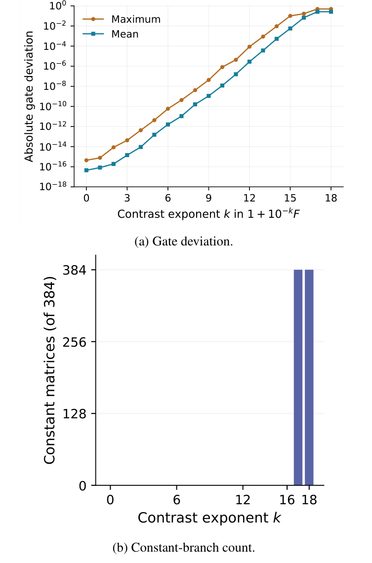
The contrast-decay experiment has no gate deviations above \(10^{-6}\) through \(k=10\). At \(k=11\), thirteen of 384 matrices exceed that threshold; at \(k=12\), the count is 96. The maximum absolute deviation reaches 0.101829 at \(k=15\) and 0.167663 at \(k=16\). Every matrix takes the constant branch at \(k=17\) and \(k=18\), with mean deviation 0.261193 from its nonconstant value. These transition points characterize the specified arrays, unit offset, and arithmetic, rather than a universal contrast threshold. They show where exact invariance ceases to describe the already rounded numerical input.
The two displays in Figure 7 distinguish increasing numerical deviations from entry into the constant branch. The first shows the mean and maximum over matrices; the second counts arrays whose centered values have become exactly zero.
The absence of constant arrays before the final two exponents does not imply negligible error: deviations grow while some contrast is still represented. Once every array is constant, the fixed convention accounts for the terminal plateau.
Individual numerical observations distinguish gradual deviations from the final numerical branch. The first threshold exceedances affect only thirteen matrices; at the final two amplitudes, every matrix is constant. The terminal mean then measures displacement from the assigned half-unit weight, rather than estimation of a residual spectrum.
Global centering removes a uniform offset, and normalization removes nonzero gain from the singular-value proportions. The resulting coefficient measures concentration, without locating contours or judging translated appearance. High horizontal-oscillation and checker weights follow from their few separable components. Their different visual frequencies are therefore compatible with similarly concentrated spectra, illustrating why intensity invariance and spatial organization require separate interpretations.
The diagonal-edge family clarifies this distinction. A coherent boundary need not have the smallest participation-ratio dimension, because oblique geometry distributes matrix energy across several separable components. Conversely, a checker pattern can have a high coefficient despite rapid changes between adjacent pixels. These observations concern the algebraic organization of the specified arrays, rather than semantic judgments about their contents. The distinction between texture sensitivity and shape sensitivity also appears in the trained classifiers studied by Geirhos et al. [19]; their findings do not imply that the present coefficient recognizes either attribute. A high value is evidence of concentration under the selected matrix representation, without an automatic interpretation as structural correctness. This interpretation also respects the separate channel and spatial operations of CBAM [10]: the present permutation result concerns the scalar channel description, not every operation that may follow it.
Independent row and column permutations preserve concentration while relocating boundaries and patterns. The unchanged coefficient cannot distinguish either photograph from its reordered counterpart. Multiplication nevertheless retains the altered arrangement: it scales the absolute difference by a common positive value and leaves the relative difference unchanged. Equal scalar weights therefore do not imply equal weighted representations.
Because centering is confined to the descriptor, the weighted channel retains its mean. Its additive transformation is \(b g(F)J\), as established analytically, and is not an illumination-corrected image. This distinction concerns the implemented map rather than a downstream prediction.
The normalized squared-gradient quantity \(D\) supplies information absent from the singular-value concentration. Across the blob and edge families, the ratios of the post-permutation mean to the pre-permutation mean are approximately 41 and 65, respectively, despite unchanged gates. These increases record the creation of differences between pixels that have become adjacent. They do not indicate improved detail. The Gaussian-noise family behaves differently: its average \(D\) changes little because the generating distribution already lacks a preferred arrangement of neighboring entries. This contrast explains why a gradient quantity can diagnose the particular rearrangement without providing a universal scale of image quality.
The photographic pairs give the same caution a directly inspectable form. Reordering the raccoon and ascent arrays increases their normalized gradient energies while visibly relocating recognizable structures. Both the unaltered and reordered arrays have exactly the same coefficient in the full-image calculations. A preference for a larger gradient value would therefore favor the altered adjacency in these cases. Fréchet inception distance addresses another question altogether: it compares image distributions through learned feature statistics [29]. Neither that distribution comparison nor the present adjacency calculation is a direct measurement of an internal coefficient’s spatial selectivity.
The used image-translation scores included in the materials establish the numerical context motivating the investigation. They do not provide the generated arrays needed to calculate this paper’s coefficient or to assess its invariance in a trained generator. They also cannot support uncertainty estimates for differences between algorithms. Chong and Forsyth show that finite-sample FID bias can depend on the generating model [30], while Parmar et al. demonstrate sensitivity to resizing and compression choices [31]. These findings make the unavailable evaluation details consequential; they do not prove that any particular availed ranking is incorrect.
The evaluation literature further distinguishes properties that one scalar can combine or overlook. Kynkäänniemi et al. assess sample quality and distribution coverage separately through improved precision and recall [32]. Naeem et al. introduce density and coverage to address particular weaknesses of preceding distribution comparisons [33]. The relevance here is methodological: a quantity intended to summarize spectral concentration should be assessed against concentration and its exact symmetries. Its numerical stability cannot substitute for evidence about image fidelity, diversity, or localization. The patch correspondence objective of CUT [5] illustrates an explicit spatial condition absent from the concentration calculation, while style-statistic alignment in adaptive instance normalization [16] uses appearance quantities that this gate intentionally removes from its descriptor.
Human judgments are likewise not recoverable from the coefficient values reported here. Stein et al. find disagreements between common Inception-based evaluations and perceived realism in their diffusion-image comparisons [34]. In a position paper, Räisä et al. argue for explicit evaluation requirements and targeted checks [35]. The present permutation test follows that narrow logic: it identifies a transformation under which the coefficient must remain equal even when adjacency changes substantially. It supplies an interpretable limitation of this operator without claiming a replacement for perceptual assessment or a ranking of image-generation methods.
The additive-noise calculation separates exact symmetry from bounded sensitivity. At relative noise norm \(0.1\), the average absolute gate change is approximately \(0.00487\), whereas the average deterministic bound is approximately \(0.206\). The inequality is therefore conservative for the sampled directions. Its value is the stated worst-case guarantee under its assumptions, rather than prediction of a typical displacement. The predominantly negative changes in the structured families are consistent with their measured concentration decreasing after the added direction distributes energy more broadly across singular components. This observed tendency is not asserted for every matrix or perturbation, and the Gaussian-noise family has changes of both signs.
The bound concerns a scalar trace ratio and requires no separation between singular values. This differs from eigenspace perturbation results, including the Davis–Kahan variant discussed by Yu et al. [36], where separation conditions govern changes of eigenspaces. Computing the gate through Gram products likewise avoids explicitly differentiating singular vectors. The issues studied by Wang et al. in differentiable SVD [37] remain relevant to other spectral layers, but avoiding those derivatives does not remove the present operator’s zero-contrast singularity. Smooth dependence away from that point and direction-dependent limits at the point are compatible mathematical properties.
The offset-dominated calculations demonstrate why this distinction matters computationally. Rescaling the centered array before evaluating its Gram concentration protects subsequent arithmetic from unnecessarily extreme magnitudes. It cannot restore contrast lost when \(1+10^{-k}F\) is first represented. In the specified calculations, all arrays reach the constant branch at \(k=17\), after substantial coefficient deviations have already appeared. This exponent depends on the offset, the stored entries, and double-precision representation; it is not a universal image-processing threshold. Moreover, the gate’s discontinuity at constants exists in exact arithmetic, whereas the observed approach to that discontinuity also includes rounding.
A numerical convention at a constant matrix completes the function definition without resolving its direction dependence. Assigning \(g=1/2\) is explicit and reproducible, but no constant assignment can supply the missing continuous extension. Adding a fixed positive denominator term would define a different operator and would change exact gain invariance. Similarly, the scalar attenuation does not estimate a covariance matrix or adjust its eigenvalues individually. Analytical nonlinear covariance shrinkage, as studied by Ledoit and Wolf [38], addresses a distinct estimation problem whose guarantees cannot be transferred to this calculation. No such estimator is implemented here.
The computational evidence is deliberately finite. The six generated families cover controlled algebraic and spatial properties, while the two photographs provide inspectable examples rather than a representative natural-image collection. Their 32 patches remain nested within two images. Repeated noise levels also share a sampled direction within each map and replicate. Accordingly, the recorded dispersions describe the executed calculations and are not independent population estimates. Common-corruption evaluation examines a wider collection of changes than affine gain and offset or norm-controlled additive directions [39]. Spatially varying illumination, clipping, camera response, compression, and predictive accuracy remain outside the established claims.
The accompanying arrays, permutation indices, seeds, and measurement files connect each numerical statement to an executable procedure. This reporting is consistent with the reproducibility concerns examined by Pineau et al. [40], while external replication has not been claimed. The mathematical contribution is correspondingly bounded: the defined spectral coefficient removes two affine-intensity degrees of freedom, retains a calculable sensitivity away from constants, and cannot identify spatial arrangement from its value. Whether that combination benefits a trained system requires a separate task-specific investigation with actual training and held-out evaluation.
Resolution and preparation remain part of the matrix definition. Cropping changes which regions contribute; interpolation introduces dependencies between entries; changing spatial dimensions changes the gate normalization. The fixed photographic processing therefore matters. The proved equalities apply to specified arrays, not to arbitrary resizing or scene preparation.
The scalar and its generating channel should consequently be interpreted together. Equal coefficients establish one reproducible property under a specified transformation, while the stored arrays permit adjacency to be examined separately. Equivalence of the images would require criteria beyond concentration.
Centered spectral concentration answers the research question in two parts. It supplies exact invariance to a nonzero global gain and arbitrary global offset, but it cannot identify spatial arrangement from its scalar value. The same singular spectrum can accompany substantially different adjacency, as demonstrated by independently permuted rows and columns in both generated matrices and recognizable photographs. Equal gate values do not erase the differences between weighted maps; they show that those differences cannot be judged from the multiplier alone.
The executed calculations locate the practical boundaries of this property. Affine differences remain at double-precision roundoff for ordinary contrast, and a relative perturbation bound covers every prescribed noise test. The bound is conservative, especially at larger disturbances. Near constant matrices, exact invariance preserves direction-dependent gate limits while finite arithmetic can discard the contrast altogether. The numerical contrast is concrete: the largest affine change across 9,600 generated-map tests is below \(7\times10^{-16}\), yet row-and-column reordering increases the mean blob difference energy by approximately forty-one times. A coefficient can therefore be exceptionally stable while the adjacency it cannot encode changes substantially.
The resulting contribution is a reproducible mathematical characterization of an explicit channel operator, supported by retained arrays and observation-level calculations. It establishes neither improved generative performance nor a preferred architecture for unpaired translation. Within its stated scope, it identifies precisely what centered spectral weighting preserves, what its scalar description cannot distinguish, and where its numerical interpretation requires nonvanishing contrast.
All data required to support the findings of this research are included in the paper.
The author declares no conflicts of interest.
This research received no external funding.
Artificial intelligence tools were used to assist with code generation and consistency checking. The author reviewed and verified all AI-assisted content and accepts full responsibility for the final manuscript.