
I. Introduction
Since the late 1990s, the concept of the urban economic circle—a spatially contiguous zone within which large and medium-sized cities share infrastructure, labour markets, production linkages, and ecological resources—has gained prominence in policy discourse from Brussels to Beijing [1], [2]. Global evidence suggests that agglomeration economies, networked transport systems, and cross-jurisdictional governance synergise to create super-regional engines of growth. In China, where the State Council formally identified urban agglomerations as “the primary form of new-type urbanisation” in 2012, the stakes are particularly high: a well-functioning urban economic circle can amplify positive spillovers, including innovation diffusion, the circulation of highly skilled talent, and supply-chain clustering, while mitigating negative externalities such as pollution, congestion, and spatial inequality [3], [4]. Uncovering the internal mechanisms of such circles—i.e., how industries are reallocated, which cities assume command-and-control functions, and how spatial proximity accelerates or impedes balanced development—therefore constitutes a pressing research agenda with direct implications for China’s dual-circulation strategy and long-term economic resilience [5], [6].
Despite four decades of rapid growth, China’s urban system remains sharply stratified. Tier-1 cities, including Beijing, Shanghai, Shenzhen, and Guangzhou, command disproportionately large shares of advanced producer services and high-technology manufacturing, whereas Tier-2 and Tier-3 municipalities often struggle to move beyond path-dependent, medium-value-added industrial activities. Peripheral Tier-5 and Tier-6 county-level cities, although occasionally supported by resource endowments or specialised tourism, typically exhibit fragmented industrial bases and weaker fiscal capacities [7], [8]. This hierarchical mosaic results in marked regional disparities: per-capita GDP in Beijing exceeded RMB 190,000 in 2023, more than six times that of many western prefectures. Consequently, the spatial distributions of manufacturing activities, services, and digital platforms exhibit heteroscedastic patterns, challenging the central government’s objective of “coordinated and balanced development,” as articulated in the 14th Five-Year Plan [9]. Although macro-level indicators—including industrial value added, employment composition, and environmental footprints—suggest systemic imbalances, the micro-spatial interplay among contiguous cities within the same agglomeration remains underexplored [10].
Scholars have long sought quantifiable proxies for industrial synergy and regional coupling. Western studies often apply the Herfindahl–Hirschman Index (HHI) to measure sectoral concentration or employ input–output matrices to trace production linkages. In China, the Theil entropy coefficient has been used to assess the rationalisation of industrial structures at the provincial level [11], [12]. Recent advances have incorporated information entropy—a Shannon-based measure that increases with distributional evenness—as a city-level indicator of industrial “balance” [13]. Parallel streams of research have explored methodological improvements, including spatial econometrics, geographically weighted regression, and, increasingly, machine-learning algorithms. Random forests (RFs), gradient boosting, and deep neural networks have demonstrated superior nonlinear predictive performance in applications involving housing prices, land-use conversion, and pollution mapping [14]. However, their application to regional industrial coupling remains at an early stage. International studies [15] have highlighted multiscalar phenomena—including firm relocation, commuting networks, and knowledge spillovers—but few have integrated city-hierarchy variables with entropy-based metrics within a machine-learning framework.
Three limitations are particularly evident in the existing body of knowledge. First, many Chinese studies rely on parametric linear regression models that assume homoscedasticity and independence, potentially misrepresenting the complex nonlinear relationships among proximity, hierarchy, and industrial composition. Second, the spatial scope is frequently restricted to individual metropolitan areas [16] or administrative units, thereby overlooking cross-regional comparability and ignoring heterogeneity among urban economic circles. Third, most analyses employ broad industrial categories, such as primary, secondary, and tertiary industries, which are insufficient for detecting subtle structural changes, including the rise of digital platforms, green manufacturing, and cultural and creative clusters. Collectively, these limitations constrain the ability to formulate precise, evidence-based policies for differentiated development pathways across China’s extensive urban hierarchy [17], [18].
Against this background, the present paper proposes a novel analytical framework that integrates (i) information-entropy-based industrial coupling indices, (ii) a random forest modelling pipeline capable of capturing high-order nonlinear interactions, and (iii) a multiscale perspective encompassing individual cities, urban economic circles, and national aggregates. By employing geospatial distances to higher-tier cities as explanatory variables alongside employment composition across six detailed industrial sectors, the study quantifies how proximity to hierarchical centres shapes industrial balance. Furthermore, the study applies K-means++ clustering to 14 nationally recognised urban economic circles, revealing latent typologies of “balanced-diversified,” “specialised-core,” and “transitioning” agglomerations. This three-layered approach not only advances the relevant methodological framework but also generates actionable insights for urban-circle-oriented governance: Which low-entropy cities require catalytic industries? Which overspecialised urban economic circles require diversification incentives? How should investments in intercity transport and digital infrastructure be prioritised?
II. Methodology
A. Two-Level Random Forest Framework for Predicting Urban Industrial Coupling
To comprehensively evaluate the nonlinear relationships between city-level spatial characteristics and their corresponding industrial coupling values, we construct a two-level random forest framework. This framework is designed to improve the predictive accuracy of the entropy-based industrial coupling index by capturing both primary mapping relationships and residual error structures [19], [20]. Figure 1 illustrates the integrated framework, which consists of three conceptual layers: the data level, task level, and method level.
At the data level, multisource and multiscale urban data are integrated to form the input feature space. These data include census information, such as urban population and employment; digital elevation models (DEMs); land-use classifications; nighttime-light imagery, which indicates the intensity of economic activity; point-of-interest (POI) distributions; and urban road networks. Collectively, these data layers reflect the spatial, functional, and socioeconomic structures of cities, thereby providing a rich set of covariates for modelling industrial development [21].
The task level defines the sequence of subtasks required to model industrial coupling. First, urban functional zones are identified using POI densities and land-use categories to delineate industrial, residential, commercial, and mixed-use areas. Subsequently, the relationships between these spatial-functional features and the target industrial entropy values are modelled. Finally, the estimated relationships are used to predict the degree of industrial coupling, represented by entropy, for each city.
At the core of the framework is the two-level random forest modelling strategy. The first-level model is a random forest regressor, denoted by \(\mathrm{RF}_1\), which is trained on the feature matrix \(\mathbf{X}\in\mathbb{R}^{n\times d}\). This matrix contains variables such as city hierarchy (\(\mathrm{Cls}\)), urban economic circle identifier (\(\mathrm{Group}\)), and distances to Tier-1 through Tier-4 cities, denoted by \((D_1,D_2,D_3,D_4)\). The model estimates the initial industrial coupling values \(\hat{\mathbf{y}}_1\) using the following mapping function:
where \(\hat{\mathbf{y}}_1\in\mathbb{R}^{n}\) is the vector of fitted coupling entropy values for \(n\) cities.
Although it captures most of the variance, the first-level prediction may still exhibit systematic residuals because of local nonlinearities or unmodelled interactions. To address this limitation, we calculate the residual errors as \(\hat{\mathbf{o}}=\mathbf{y}-\hat{\mathbf{y}}_1\), where \(\mathbf{y}\) denotes the vector of observed entropy values. A second-level random forest model, denoted by \(\mathrm{RF}_2\), is subsequently trained to model these residuals:
The final industrial coupling prediction \(\hat{\mathbf{y}}\) is obtained by summing the predictions produced at the two levels:
This hierarchical prediction strategy ensures that both the dominant structural patterns and finer-scale deviations are captured, thereby enhancing the accuracy and generalisability of the model.
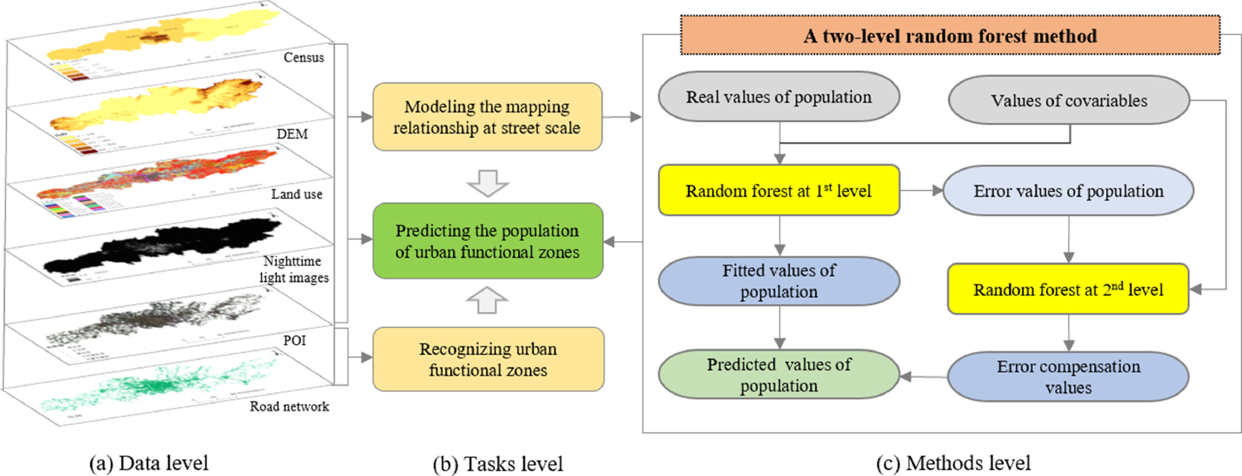
Figure 1 graphically summarises the entire analytical procedure. On the left, the data-level layers illustrate the variety of spatial and socioeconomic data integrated into the model. The central column presents the sequential tasks of spatial-functional recognition and entropy mapping. The right-hand panel presents the method level and details the two-stage learning process, which consists of initial entropy fitting followed by residual error compensation using random forests.
This two-level framework offers several advantages. First, it effectively mitigates the limitations of single-stage models, particularly in complex spatial domains containing multicollinear features. Second, it preserves model interpretability by allowing feature importance to be estimated at both levels of the framework. Finally, its modular structure enables the flexible integration of additional covariates or urban data layers, making the framework extensible to multiregional analyses conducted across diverse urban contexts.
The accuracy and representativeness of any machine-learning-based spatial analysis depend heavily on how the input data are sampled from the underlying spatial surface. In the context of urban industrial coupling analysis, a major challenge involves selecting representative samples from heterogeneous urban regions that exhibit complex spatial distributions of industry, infrastructure, and population.
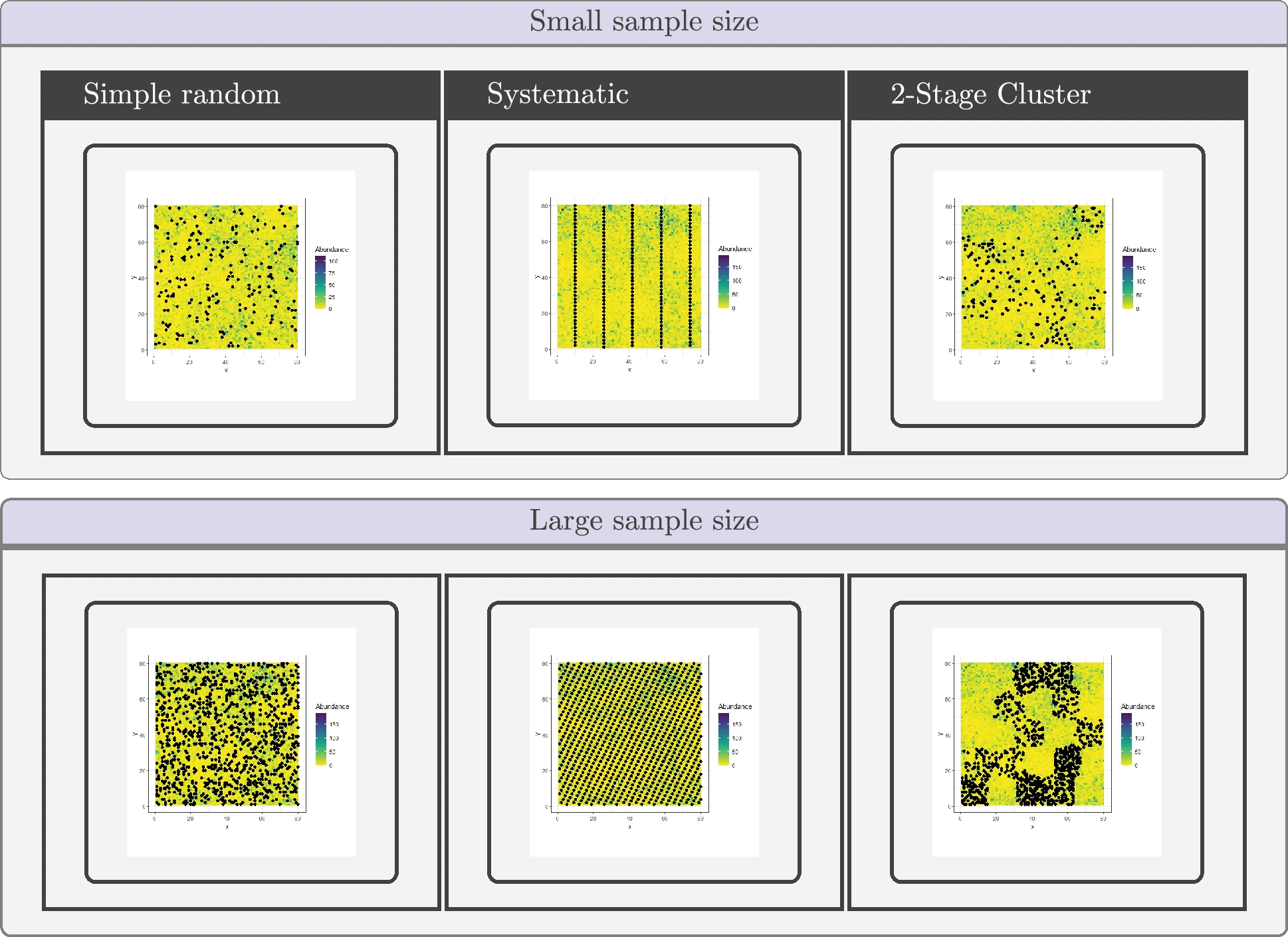
To address this challenge, the present study evaluates and integrates three classical sampling strategies under different sample-size constraints: simple random sampling, systematic sampling, and two-stage cluster sampling. These sampling strategies are illustrated in Figure 2 under both small- and large-sample settings.
1) Simple Random Sampling
Simple random sampling (SRS) selects a fixed number of spatial units uniformly and randomly across the entire study area. This method has the advantages of statistical simplicity and unbiasedness; however, it may inadequately represent spatial clusters or specific functional subregions.
Mathematically, the probability of selecting a unit \(x_i\in X\) is expressed as follows:
where \(N\) is the total number of available sampling units. This method provides the following unbiased estimator of the spatial mean:
where \(y_i\) represents the entropy or industrial value observed at sampling point \(x_i\).
2) Systematic Sampling
Systematic sampling involves selecting units at regular intervals from an ordered list or spatial grid. In a spatial context, this procedure commonly involves the construction of a uniform grid from which every \(k\)-th unit is selected.
Let the sampling interval be \(k=\frac{N}{n}\). The sampled spatial units are then given by
This method ensures relatively uniform spatial coverage but may introduce bias when periodic spatial patterns coincide with the sampling grid, as illustrated in the middle column of Figure 2. Its principal strength is its ability to provide higher precision for large samples in areas characterised by regular land-use structures.
3) Two-Stage Cluster Sampling
In two-stage cluster sampling, spatial units are organised into primary clusters, such as subregions or administrative districts, from which a subset of clusters is initially selected. Subsequently, a set of sampling points is drawn from within each selected cluster.
Let \(C\) denote the total number of clusters and \(M\) denote the number of secondary units within each cluster. During the first stage, \(c\) clusters are selected from the \(C\) available clusters. During the second stage, \(m\) samples are drawn from each selected cluster.
The resulting estimator is expressed as follows:
This sampling method is suitable for representing functional zones, including commercial or industrial blocks, and facilitates cost-effective field-data collection. It can also preserve information concerning spatially concentrated urban functions that might otherwise be inadequately represented by sampling procedures that disregard the underlying cluster structure.
As shown in Figure 2, when the sample size is small, simple random sampling and two-stage cluster sampling provide better spatial representativeness in heterogeneous regions. Under large-sample conditions, systematic sampling ensures optimal coverage in uniformly distributed areas. However, in urban contexts characterised by strong clustering of industrial features, two-stage cluster sampling emerges as a robust and scalable solution, particularly when it is integrated into functional-zone-based entropy modelling.
B. K-Means++ Clustering of Urban Economic Circles
To reveal common structural patterns and typologies among China’s diverse urban economic circles, we perform a clustering analysis based on city-level and zone-level industrial characteristics [22]. The objective is to group urban economic circles that exhibit similar internal industrial coupling structures and hierarchical compositions, thereby identifying latent regional development pathways.
1) Clustering Dimensions and Feature Construction
The clustering analysis is conducted using a set of indicators aggregated at the level of the urban economic circle, with each urban economic circle treated as an individual clustering unit. Three principal groups of features are constructed.
The first group represents the proportion of cities at each hierarchical level, from Tier 1 to Tier 6, within each urban economic circle. For a given urban economic circle \(g\), the proportion of Tier-\(k\) cities is defined as follows:
where \(n_{gk}\) is the number of Tier-\(k\) cities in urban economic circle \(g\), and \(n_g\) is the total number of cities within that circle.
The second group represents the average proportion of employment in major industries, such as manufacturing, construction, trade, and transportation, aggregated across all cities within each urban economic circle:
where \(E_{ji}\) is the number of people employed in industry \(i\) in city \(j\), and \(E_j\) is the total number of employed people in city \(j\).
The third group represents the average industrial coupling value \(\overline{H}_g\) calculated across all cities within each urban economic circle:
All features are standardised using \(z\)-score normalisation to eliminate differences in measurement scales:
C. K-Means++ Algorithm and Initialisation
We apply the K-Means++ algorithm to perform the clustering analysis. This algorithm improves upon the standard K-Means method by enhancing the initial selection of cluster centroids, thereby promoting better convergence and producing more stable clustering results.
Given a data matrix \(\mathbf{X}\in\mathbb{R}^{m\times d}\), containing \(m\) urban economic circles and \(d\) standardised features, the K-Means objective function is expressed as follows:
where \(C_k\) is the set of urban economic circles assigned to cluster \(k\), and \(\boldsymbol{\mu}_k\) is the centroid of cluster \(k\).
The K-Means++ initialisation procedure selects the first centroid randomly and selects the remaining centroids probabilistically according to their squared distances from the existing centroids. This procedure promotes a wider initial distribution of centroids and reduces the likelihood that the algorithm will converge to a poor local minimum.
D. Determination of the Optimal Value of \(K\)
To determine the optimal number of clusters, \(K\), we employ two widely accepted approaches: the elbow method and the silhouette coefficient.
For the elbow method, we calculate the total within-cluster sum of squares (WCSS) across a range of values \(K\in[2,10]\). The “elbow point,” at which the rate of decline in the WCSS decreases sharply, indicates a reasonable balance between explained variation and model parsimony.
For the silhouette-coefficient method, we calculate the silhouette score \(S\in[-1,1]\) for each candidate value of \(K\). This score reflects both within-cluster cohesion and between-cluster separation:
where \(a\) is the average intracluster distance and \(b\) is the average distance to the nearest alternative cluster. A higher silhouette score indicates more clearly defined and better-separated clusters.
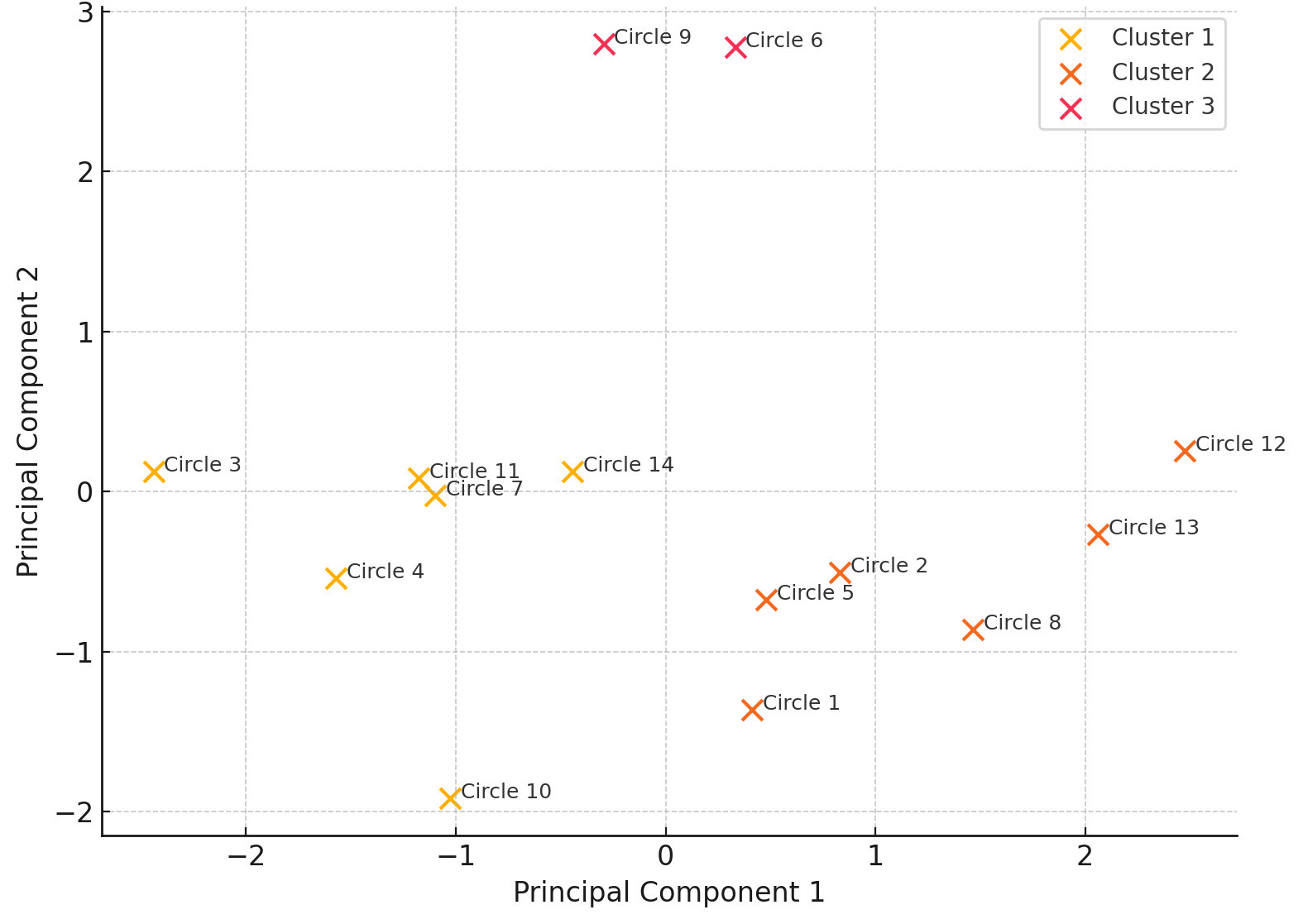
Based on the elbow plot and the trend in the silhouette scores, \(K=3\) is selected as the optimal number of clusters because it provides an appropriate trade-off between interpretability and internal consistency. These results are illustrated in Figure 3, in which the three clusters reveal distinct structural patterns in the compositions and industrial roles of the urban economic circles. The plot presents 14 urban economic circles projected onto two principal components through principal component analysis (PCA). Each urban economic circle is assigned to one of the three clusters, labelled Clusters 1–3, distinguished by colour, and identified as “Circle 1” through “Circle 14.”
III. Results and Discussion
A. Indicator Description and Data Status
In recent years, most studies have used the Theil index as an indicator of the rationalisation of industrial structures. However, this approach presents several problems. First, it is generally based only on the primary, secondary, and tertiary sectors and therefore does not reflect the more detailed classification of industries at the national level [23], [24]. Second, this indicator is more appropriate for studying individual cities. When the research target is an urban agglomeration, its application becomes less convenient because of factors such as limited data availability and differences in statistical standards. The specific industries examined in this study are described in Table 1.
| Statistic | Particular year | Agriculture, forestry, animal husbandry, and fishery | Mining industry | Manufacturing | Construction | Restaurant | Trade | Transport |
|---|---|---|---|---|---|---|---|---|
| Count | 2000 | 3965 | 3778 | 3998 | 3995 | 3557 | 3587 | 3994 |
| Mean | – | 1.1 | 1.89 | 13.05 | 1.01 | 5.34 | 1.96 | 0.7 |
| Std | – | 3.55 | 3.04 | 20.69 | 0.86 | 9.74 | 4.23 | 2.97 |
| Min | 2004 | 0 | 0 | 0.06 | 0 | 0 | 0 | 0 |
| 25% | – | 0.15 | 0.13 | 0.14 | 0.57 | 0.17 | 0.54 | 0.14 |
| 50% | – | 0.85 | 0.47 | 6.4 | 0.81 | 1.69 | 0.87 | 0.57 |
| Max | 2016 | 95.58 | 20.72 | 258.8 | 11.08 | 134.98 | 60.79 | 69.22 |
In this paper, information entropy is used as a measure of industrial rationalisation. Information entropy is a commonly used metric in traditional machine-learning algorithms for measuring the purity or uncertainty of an ensemble.
The formula for information entropy is expressed as follows:
A higher value indicates a higher degree of balanced industrial development and stronger industrial coupling within the region.
The data used for the industrial structure analysis were obtained from the China Statistical Yearbook for the period 2003–2016. This study uses the number of people employed in different industrial categories, measured in units of 10,000 persons, to represent the industrial development of a city. Let \(K_{y,c}\) denote the proportion of people employed in industry \(i\) in city \(c\) at the end of year \(y\) relative to the total number of people employed in that city during the same year. The industrial coupling value is then calculated as follows:
The descriptive statistics for the data are presented in Table 1. Representative industrial categories and their corresponding numbers of employees are used to characterise the development of different industries within each city.
B. Data Sources and Preprocessing
This study utilises city-level panel data obtained from the China Statistical Yearbook for the period 2003–2016. The data encompass variables such as urban administrative hierarchy (\(\mathrm{Cls}\)), industrial employment across six core sectors, urban agglomeration membership (\(\mathrm{Group}\)), and geographical proximity to higher-tier cities (\(D_1\)–\(D_4\)). To ensure model robustness and interpretability, a comprehensive data-preprocessing and modelling pipeline is implemented, as illustrated in Figure 4.
The raw data undergo categorical encoding using LabelEncoder for discrete variables such as city levels and urban groups. Continuous variables, including industrial proportions and spatial-distance metrics, are standardised using \(z\)-score normalisation to eliminate scale-related biases and stabilise model convergence. The processed data are subsequently divided into training and testing subsets, accounting for 70% and 30% of the observations, respectively. Five-fold cross-validation is employed during model training to assess and improve generalisation.
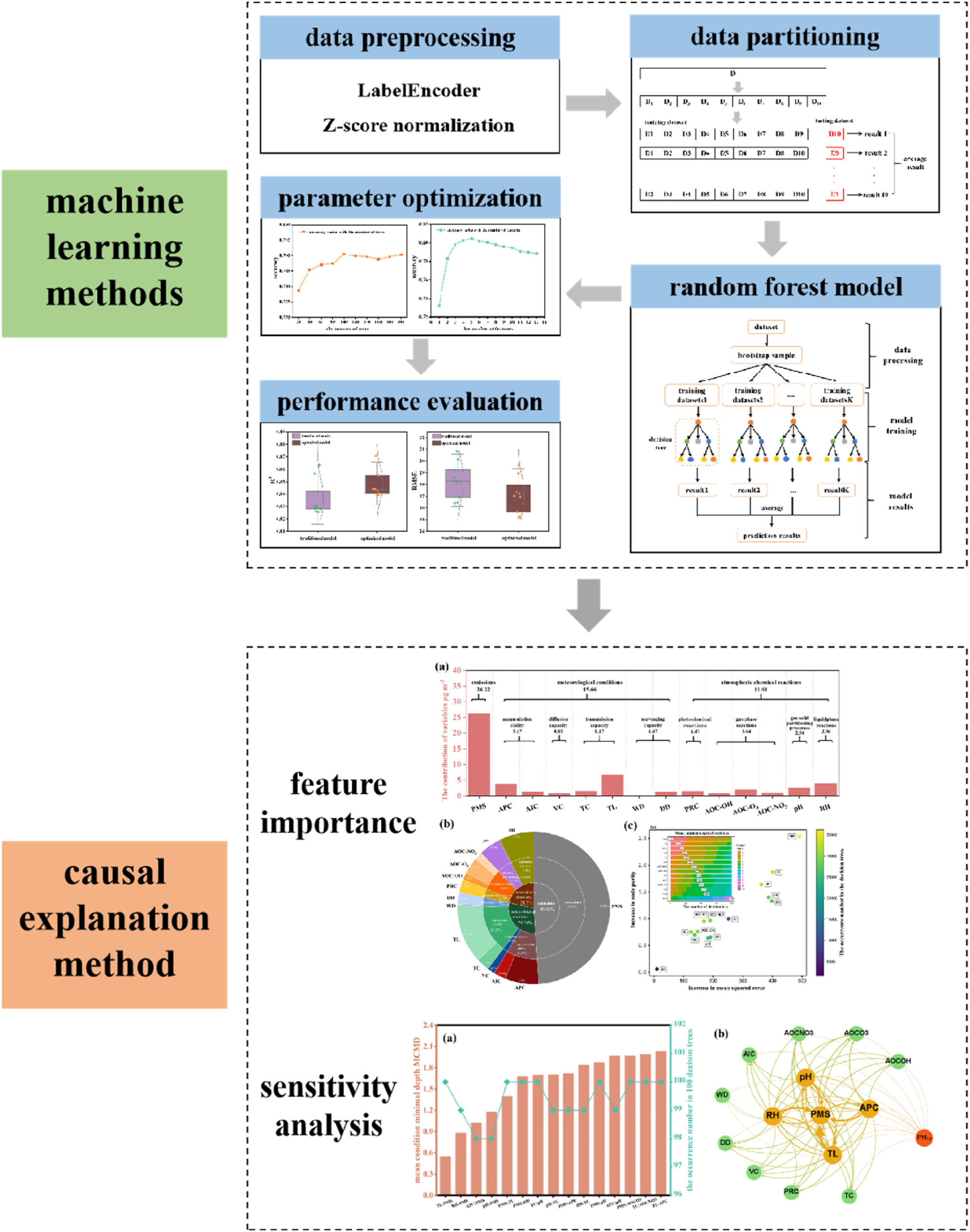
A random forest regression model is adopted, and its principal hyperparameters, including the number of trees, the maximum number of features considered at each split, and tree depth, are optimised through a grid-search procedure based on the minimisation of the mean squared error (MSE). Following model fitting, predictive performance is evaluated through residual analysis and boxplots comparing the training and testing errors.
To extend the analysis beyond predictive accuracy, post hoc interpretation methods are also applied. Feature importance is quantified using mean decrease in impurity (MDI), revealing that proximity to Tier-2 and Tier-3 cities plays a dominant role in shaping industrial coupling outcomes. Sensitivity analysis is then used to examine how marginal changes in individual features affect the predicted entropy values. This integrated framework ensures that the predictive model is not only accurate but also explainable, thereby providing a solid foundation for the subsequent clustering analysis and regional policy recommendations.
C. Comparative Model Performance
As shown in Figure 5, four geographically separated cities at different hierarchical levels were randomly selected. The capitalised numbers presented in parentheses indicate the corresponding city levels, while the figure illustrates the distribution of employment across industries within the selected cities. The general patterns of industrial development in the four cities are relatively similar, although clear differences in their employment distributions can also be observed. Changsha and Xi’an have relatively high proportions of manufacturing employment, whereas Haikou has the highest proportion of construction employment and a comparatively low proportion of manufacturing employment.
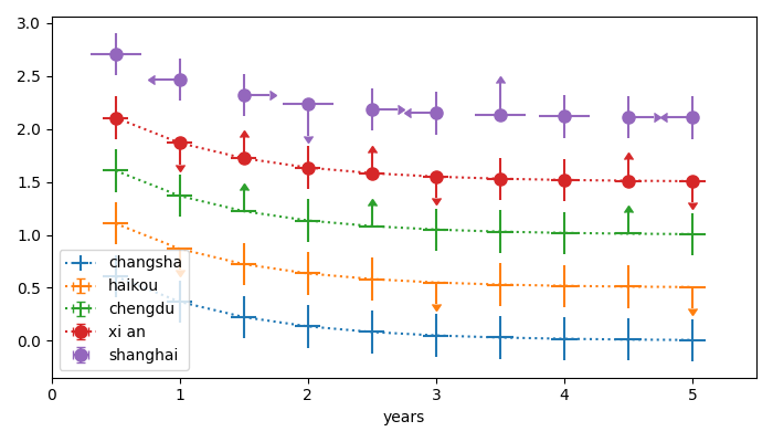
The average industrial coupling values calculated for the four cities in 2010 were 2.31 for Chengdu, 2.384 for Xi’an, 2.407 for Changsha, and 2.95 for Haikou. These values are consistent with the patterns presented in Figure 5. It should also be noted that the industrial distributions of the two Tier-3 cities, Xi’an and Changsha, are highly similar. By contrast, the distributions observed for the Tier-2 city of Chengdu and the Tier-5 city of Haikou differ considerably from one another.
To further validate the robustness and transferability of the industrial coupling prediction framework within urban economic systems, we compare the performance of six machine-learning models on the task of urban population estimation, which is strongly associated with industrial scale and structural balance. Figure 6 presents scatterplots of estimated population values against actual census population values across all testing samples, highlighting prediction accuracy, linear fitting trends, and the coefficient of determination.
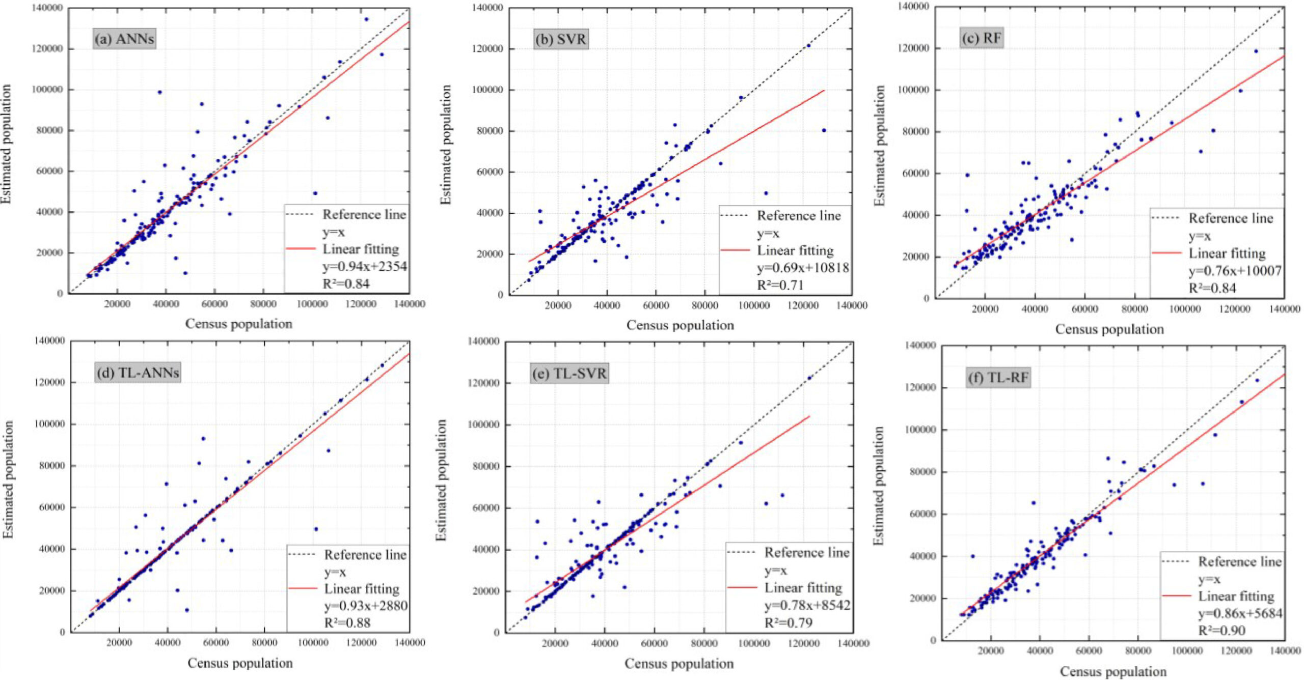
Figure 6(a) presents the baseline performance of a conventional artificial neural network (ANN) model, which achieves an \(R^2\) value of 0.84. Figure 6(b) demonstrates the lower predictive performance of support vector regression (SVR), which achieves an \(R^2\) value of 0.71. In Figure 6(c), the random forest (RF) model demonstrates improved alignment between the predicted and actual values, with an \(R^2\) value of 0.84, thereby supporting the suitability of tree-based methods for spatially structured data.
More importantly, the bottom row, comprising Figure 6(d)–Figure 6(f), present the transfer learning (TL)-enhanced versions of the three models. In these models, knowledge obtained from pretrained models or auxiliary datasets is incorporated to improve generalisation. The TL-ANN model in Figure 6(d) increases the \(R^2\) value to 0.88, whereas the TL-SVR model in Figure 6(e) improves the value to 0.79. The strongest result is obtained by the TL-RF model in Figure 6(f), which achieves a substantially improved \(R^2\) value of 0.90 and a linear fitting relationship of \(y=0.86x+5684\). These results indicate both higher predictive accuracy and reduced systematic bias.
The observed performance trends confirm that tree-based models, including RF and TL-RF, outperform the kernel-based SVR model. This advantage is likely attributable to their ability to capture high-order interactions among urban characteristics, such as industrial employment proportions and spatial distances. The results also demonstrate that transfer learning substantially improves model performance, particularly in small-sample or domain-shift contexts, which are frequently encountered in cross-regional urban modelling.
To further improve the generalisation ability and spatial adaptability of the urban regional industrial coupling model, this study systematically evaluates model bias under conditions of high and low spatial autocorrelation using different spatial sampling and cross-validation strategies, as shown in Figure 7. As a highly spatially organised regional unit, an urban economic circle often exhibits pronounced internal agglomeration and hierarchical characteristics. This pattern is particularly evident in representative urban economic circles such as the Beijing–Tianjin–Hebei region and the Yangtze River Delta, both of which exhibit high levels of spatial autocorrelation.
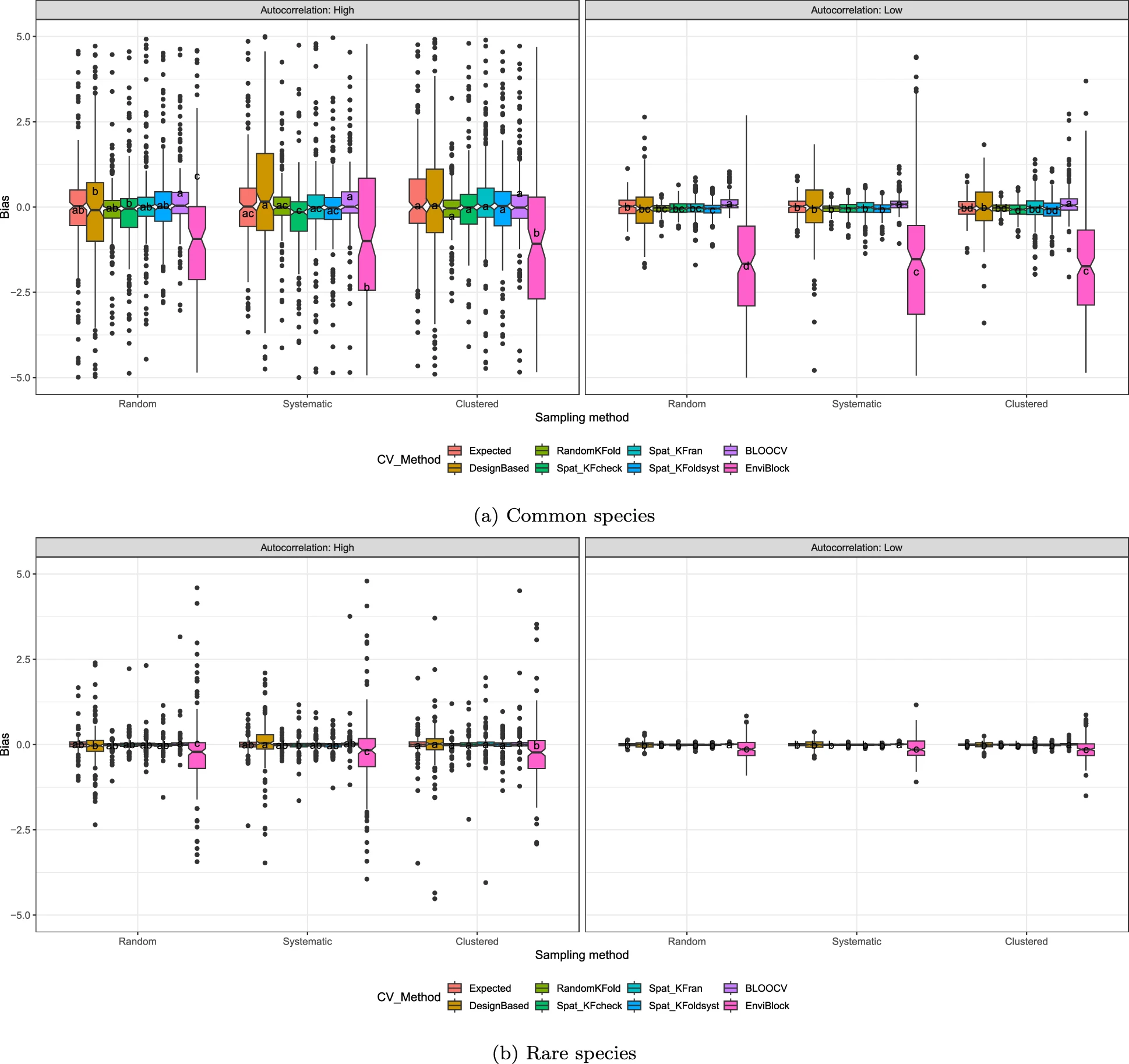
The experimental results show that conventional RandomKFold cross-validation is prone to overfitting under conditions of high spatial autocorrelation. This tendency is particularly evident when clustered sampling is employed, as the distribution of model bias becomes substantially wider. Spatially aware validation methods, such as Spat_KFoldCheck and EnvBlock, can effectively control model bias. Their performance is particularly strong in urban regions containing substantial internal structural differences, such as differences between core cities and peripheral nodes.
By contrast, in regions characterised by low spatial autocorrelation, including certain inland urban areas and regions with decentralised industrial structures, the differences among the validation methods tend to become smaller. Nevertheless, the spatial-blocking method, EnvBlock, continues to maintain the lowest systematic bias, indicating that it is broadly applicable to spatial units characterised by uneven distributions. Its performance suggests a stronger capacity for general adaptation across heterogeneous and spatially unbalanced urban units.
Furthermore, when structurally uncommon or atypical urban areas are simulated, such as the middle reaches of the Yangtze River and the Chengdu–Chongqing Economic Circle, the influence of validation strategies on model stability becomes more pronounced. This result emphasises the importance of adopting spatially sensitive validation strategies when modelling heterogeneous urban regions.
Figure 8 presents the multi-indicator prediction results and corresponding error distributions, thereby evaluating the robustness and generalisation ability of the urban economic circle industrial coupling regression model across multiple categories of indicators. The left-hand side of the figure compares the observed and predicted values of representative variables, including CO\(_2\) emissions, CO, NO\(_x\), HC, and FC. The results show that most of the predicted points, represented by purple crosses, are distributed around the actual values, represented by black lines. This distribution indicates that the model exhibits relatively strong stability when addressing variations in industrial development among different regions.
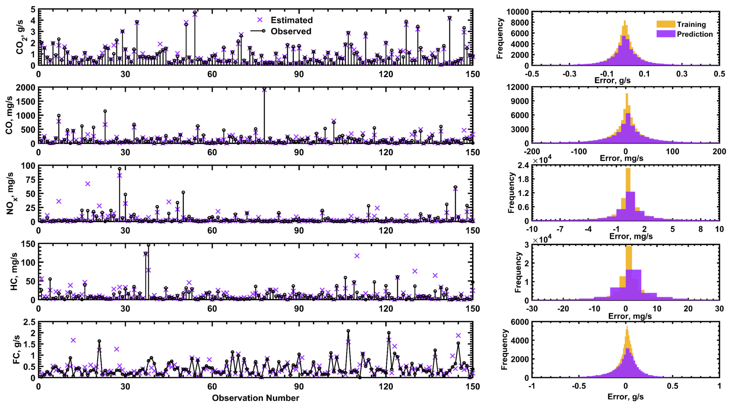
Among the examined variables, CO\(_2\) and FC (fuel consumption), which serve as representative indicators of industrial scale and energy-consumption levels within urban areas, exhibit particularly smooth fitted curves, with \(R^2\) values exceeding 0.85. The individual prediction deviations observed for NO\(_x\) and HC may result from nonlinear disturbances caused by fluctuations in the proportions of transportation and secondary industries within urban areas. These deviations reflect the industrial restructuring processes occurring in small- and medium-sized cities and their varying capacities to satisfy urban energy-consumption requirements. They also demonstrate the heterogeneity of small- and medium-sized cities in terms of industrial reorganisation and patterns of energy use.
The right-hand side of Figure 8 presents histograms of the training and testing errors for each indicator, with the training errors shown in orange and the testing errors shown in purple. All error distributions are approximately normal, and most are concentrated around zero, indicating that the model does not exhibit substantial underfitting or overfitting. The error distributions for CO and HC are relatively flat, suggesting that fluctuations in these variables are more likely to be influenced by heterogeneous industrial structures within urban areas. By contrast, the error distributions for CO\(_2\) and FC are sharper, indicating that the model is more stable when fitting indicators representing the overall scale of industry. This stability is particularly important for predicting industrial coupling entropy.
Figure 9 shows differences in model performance when predicting CO\(_2\), CO\(_x\), NO\(_x\), HC, and FC across 18 categories of urban economic subgroups. The mean bias error (MBE) is presented on the horizontal axis, while the root mean square error (RMSE) is presented on the vertical axis. These two measures are used to evaluate systematic errors and the dispersion of errors across the different categories of cities.
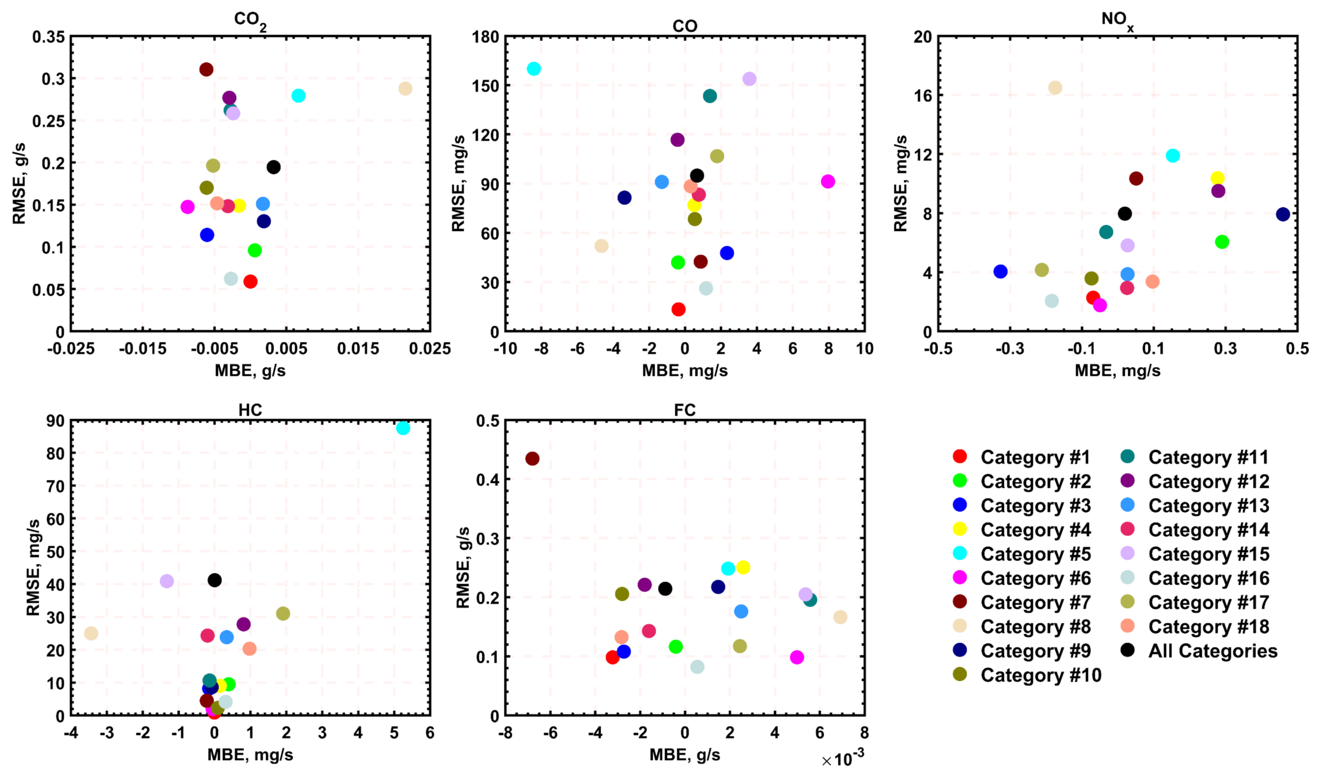
The five subfigures demonstrate that substantial differences exist in industrial coupling characteristics and model generalisation ability among the different types of urban economic regions, represented by Categories #1–#18. These differences have practical significance for developing locally appropriate industrial optimisation strategies for different types of urban regions.
In the predictions of CO\(_2\) and FC, most categories are concentrated within the low-bias and low-RMSE region, indicating that energy-consumption indicators can be modelled with relatively stable performance across different categories of cities. However, certain city categories, such as Categories #6 and #12, deviate from the principal clusters and exhibit systematic underestimation or overestimation by the model. These deviations may arise from the distinctive characteristics of these cities in terms of fuel-use structures, the carbon intensity of transportation, or their underlying demographic composition.
Differences in the modelling performance of CO\(_x\) and NO\(_x\) are even more pronounced. Multiple categories are distributed across the MBE axis, with some categories exhibiting concentrated negative bias, such as Categories #2 and #14, while others are skewed towards positive errors, such as Categories #11 and #16. These patterns suggest that the functional division of labour among industries within metropolitan areas, the pollution characteristics of dominant industries, and differences in regional atmospheric background conditions exert structural effects on the model results.
Figure 10 presents the K-Means++ clustering results for the coupled industrial characteristics of urban economic circles under different numbers of clusters, ranging from \(K=2\) to \(K=5\). The horizontal and vertical axes represent the first two principal components, which cumulatively explain approximately 87% of the variance in the original variables and therefore possess strong structural discriminatory power.
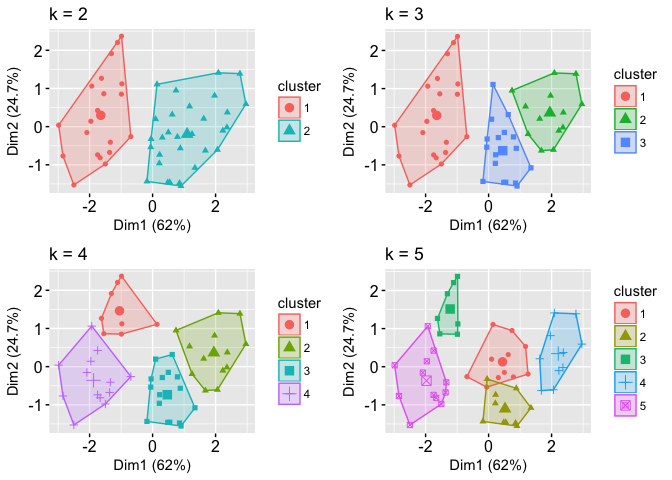
As shown in Figure 10, when \(K=2\), the urban economic circles are divided into two broad categories corresponding to highly synergistic core circles and loosely structured non-core regions. Although this division is relatively simple, considerable heterogeneity remains within the identified categories. When \(K=3\), representative moderately coupled regions, including Chengdu–Chongqing, Changsha, and other emerging urban economic circles, are further distinguished.
The clustering results obtained when \(K=4\) demonstrate improved structural discrimination and a better balance within the clusters. The first category represents highly coupled eastern regions, the second represents medium-ranked inland urban economic circles, the third comprises structurally active but lower-ranked regions, and the fourth may represent resource-dependent or peripheral urban economic circles. When \(K=5\), the category of peripheral cities is divided more precisely; however, the numbers of observations within the clusters become unbalanced, and cluster stability declines.
Therefore, \(K=4\) is identified as the optimal number of clusters. This solution not only enables the hierarchical identification of urban economic circle structures but also provides a classification basis for formulating differentiated regional development policies. It may consequently support the systematic governance of industrial coupling and synergistic mechanisms within urban economic circles.
D. Analysis of Urban Economic Data
Figure 11 presents the spatial distributions of two principal economic and social indicators within the city in 2014: the Socioeconomic Index (SEI) and the Herfindahl–Hirschman Index (HHI). The SEI map represents the level of comprehensive socioeconomic development across different areas of the city based on education, income, and employment. The transition from darker to lighter blue represents a change from higher to lower socioeconomic levels. The HHI map measures the concentration of regional industrial or demographic structures. Higher HHI values indicate the greater dominance of a particular economic factor within a region and therefore reflect a higher degree of homogeneity in the regional economic structure.
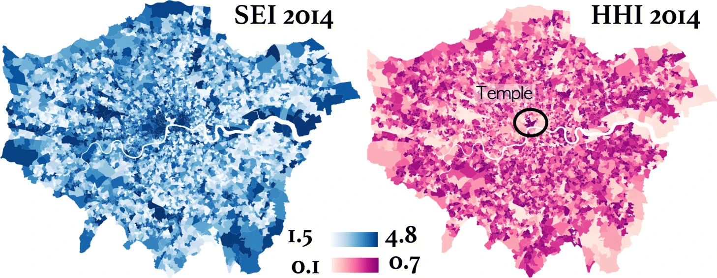
The SEI map shows that the central urban area and the eastern riverside zone exhibit higher levels of socioeconomic development. These patterns may be attributable to the concentration of policy resources in the central city, well-developed infrastructure, and the concentration of high-income residents in central areas. By contrast, peripheral areas, including the southwestern and northeastern sections, demonstrate relatively low levels of socioeconomic development, suggesting that a certain degree of uneven development exists within the urban economic circle.
The HHI map reveals highly concentrated characteristics in the Temple area, indicating that a particular industry or demographic group is strongly dominant in this area and that structural homogeneity may be present. Overall, HHI values in the central urban area are generally higher than those in peripheral areas. This pattern indicates that proximity to the urban core is associated with a greater concentration of dominant economic activity, whereas the urban periphery exhibits a more diversified structure.
Figure 12 illustrates the distribution of spatial connectivity intensity based on geographical proximity within cities in 2014. Lines of different colours represent varying strengths of connections among regions. Red lines, with values exceeding 0.995, represent the strongest spatial coupling, while orange lines, ranging from 0.99 to 0.995, and yellow lines, ranging from 0.95 to 0.99, represent moderate and weaker connection strengths, respectively.
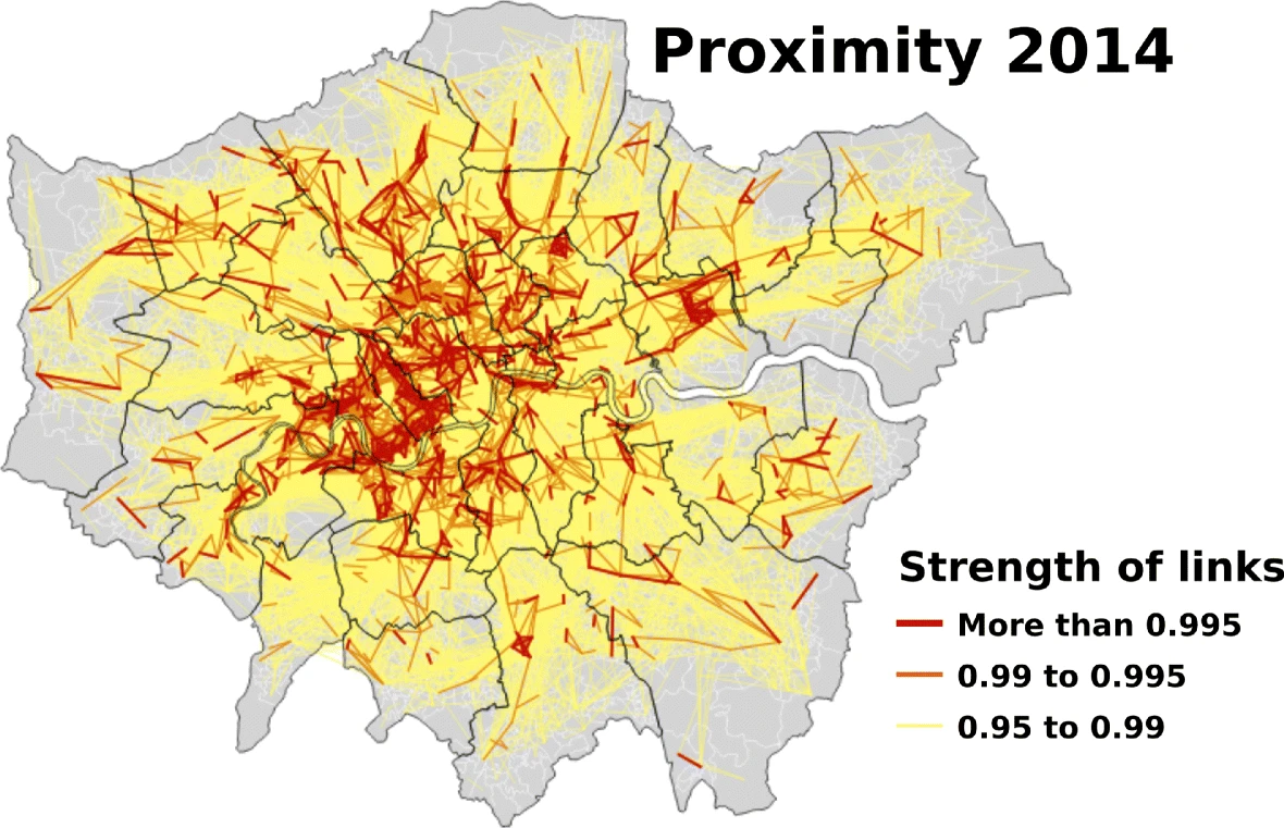
The Figure 12 demonstrates that spatial connections within the urban core are the most intensive and form a highly agglomerated network structure. This pattern reflects the pivotal role played by these areas within the urban economic circle, including their involvement in frequent industrial collaboration, transportation flows, and commercial interactions. Peripheral urban areas extend radially towards the centre, demonstrating a degree of functional dependence and commuting synergy. This distribution represents a typical “centre–periphery” spatial structure.
By contrast, the strengths of connections among peripheral areas are noticeably weaker. Their sparse spatial interactions suggest that these areas remain marginalised within the urban economic circle or require further development. The observed differences in connectivity therefore reflect an uneven distribution of economic activity, accessibility, and functional integration within the wider urban system.
Figure 13 illustrates the spatial distribution of core functional nodes in Figure 13(A) and the spatial expansion pattern of industrial agglomeration in Figure 13(B) within the London Urban Economic Circle in 2014. The analysis seeks to reveal structural evolution and agglomeration mechanisms within the urban economic circle through the high-frequency connectivity relationships between enterprise distributions and the broader economic network.
Figure 13(A) shows that core business nodes, including Temple, Tottenham Court Road, Marylebone, and London Bridge, not only have high densities of enterprises but also function as hubs that radiate towards multiple surrounding locations. These characteristics reflect the strong gravitational influence and outward connectivity of these areas within the city’s economic activities.
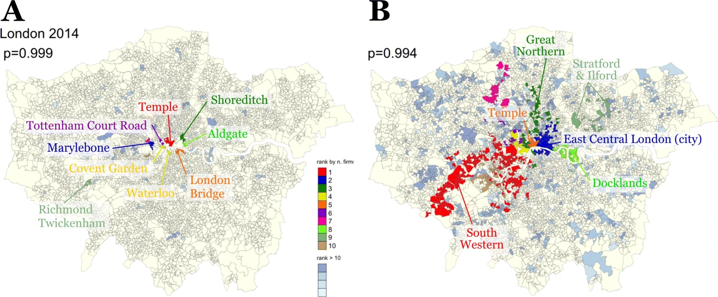
Figure 13(B) further depicts industrial clusters centred on East Central London, South Western London, and the Docklands. These clusters form several functional subcircles through the division of labour along industrial chains, high-density concentrations of enterprises, and geographical proximity. They therefore demonstrate the “polycentric” and “clustered” characteristics of the wider urban economic circle.
The colour-coded enterprise rankings in Figure 13 highlight differences in the intensity of activity among regions within the urban economic network. Red areas represent the most densely clustered core zones, whereas grey-blue areas represent secondary economically active zones or peripheral regions. This ranked structure not only reflects interactions between dominant industries and spatial organisation but also reveals the unevenness of the spatial economy and the tendency for resources to become concentrated in central areas.
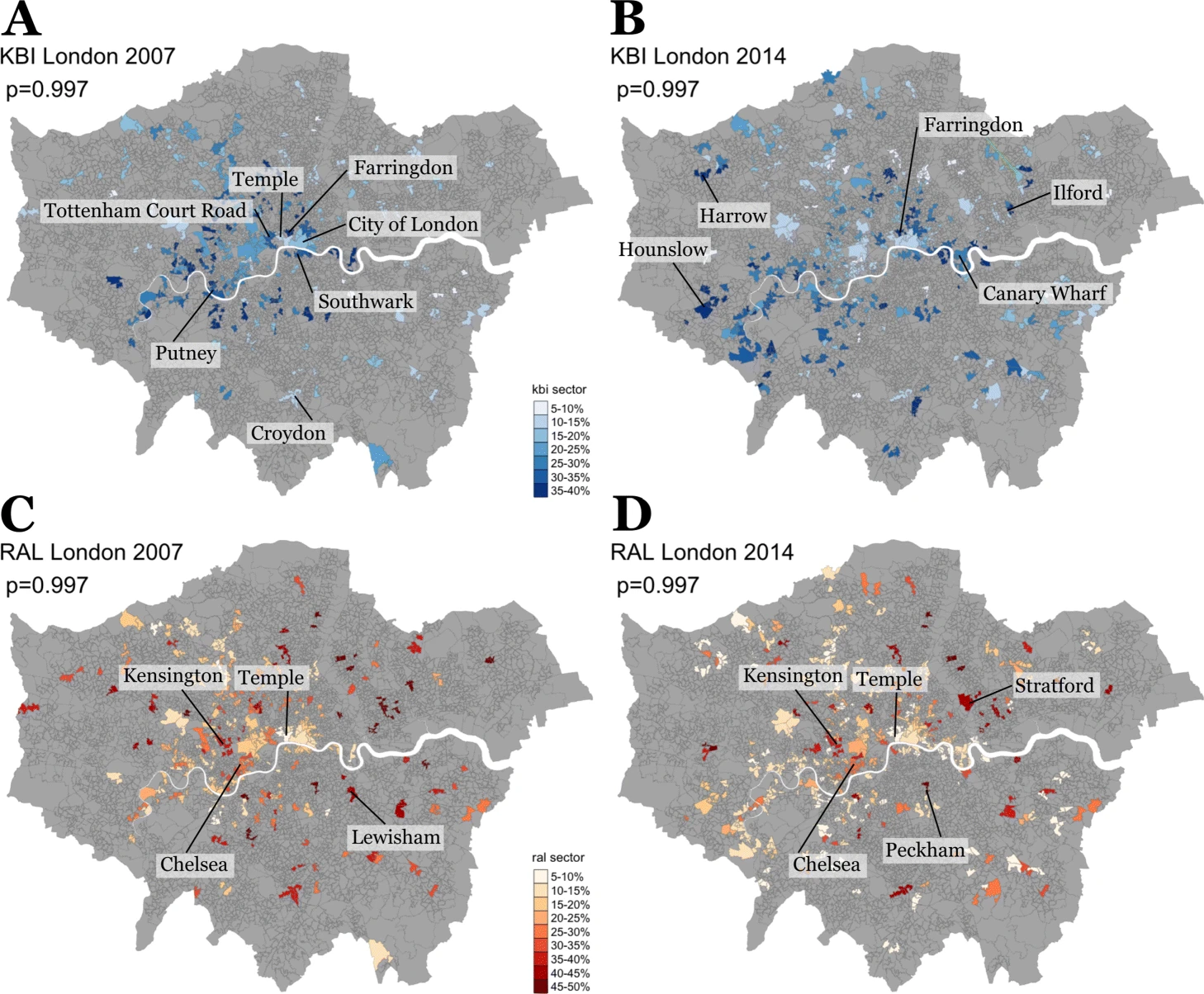
Figure 14 illustrates the spatial evolution of two important categories of industries—knowledge-intensive industries (KBI) and retail, arts, and leisure (RAL)—within the London Urban Economic Area between 2007 and 2014. In particular, Figure 14(A) and Figure 14(B) present the distribution patterns of KBI in 2007 and 2014, respectively, with darker areas indicating higher proportions of this category of industry.
The gradual transition from concentrations in central areas such as Temple, the City of London, and Tottenham Court Road in 2007 to expansion towards secondary centres such as Harrow, Hounslow, and Canary Wharf in 2014 indicates that knowledge-intensive industries are shifting from “core concentration” towards “multicentre diffusion.” This pattern suggests that the spatial organisation of knowledge-intensive economic activity is becoming less dependent on a single central core and increasingly distributed across multiple urban nodes.
The RAL distributions presented in Figure 14(C) and Figure 14(D) reveal the spatial dynamics of the consumption and leisure industries. These activities were concentrated in high-income areas such as Kensington and Chelsea in 2007 but had expanded into peripheral urban areas such as Peckham and Stratford by 2014. This structural transition highlights an evolutionary mechanism of “industrial functional differentiation–functional superposition–spatial reorganisation” within the urban economic circle. The observed pattern supports the broader trend towards increased coupling and the formation of a multinodal network structure within the urban economic circle.
IV. Conclusions
This study presents an integrated and scalable analytical framework for evaluating the structural characteristics and industrial coupling levels of China’s regional urban economic circles. By employing a two-level random forest regression pipeline, the framework accounts for complex nonlinear interactions between urban spatial characteristics and industrial entropy, thereby addressing important limitations in previous econometric assessments of industrial coupling.
The model demonstrates strong predictive performance and interpretability, particularly in identifying how proximity to cities at different hierarchical levels and industrial diversity contribute to regional synergy. The entropy-based industrial coupling index captures subtle structural variations that cannot be adequately represented by broad primary–secondary–tertiary industrial classifications. It therefore enables the detection of nuanced development trends, including the emergence of cultural and creative clusters and digital service centres.
The incorporation of spatially aware sampling and validation techniques, including two-stage cluster sampling and Spat_KFold, substantially improves model generalisation across heterogeneous categories of cities. These methods are especially valuable in regions exhibiting strong spatial autocorrelation, where conventional random cross-validation approaches may underestimate prediction errors or generate misleading assessments of model performance.
The clustering analysis identifies three dominant urban economic circle typologies: balanced-diversified, specialised-core, and transitioning. Each typology carries distinct implications for regional planning and industrial policy. Balanced-diversified urban economic circles may serve as benchmarks for integrated and coordinated development, whereas overspecialised regions require strategic incentives to promote industrial diversification. Transitioning regions require catalytic investment in digital technologies, green industries, infrastructure, and human capital to strengthen their long-term development trajectories.
Overall, the proposed framework provides a flexible and interpretable approach to analysing industrial coupling across urban economic circles. It also offers an empirical basis for differentiated regional policies concerning industrial restructuring, infrastructure investment, spatial coordination, and sustainable urban development.
Data Availability
The raw data supporting the findings of this study are available from the author upon reasonable request, without undue restriction.
Conflicts of Interest
The author declares that there are no conflicts of interest regarding the publication of this work.
Funding Statement
This research received no specific grant or financial support from any funding agency in the public, commercial, or not-for-profit sectors.