
I. Introduction
An industrial decision can be consequential even when the numbers supporting it appear modest. A manufacturer choosing between access to artificial intelligence, ethical oversight, internal analytical expertise, and investment justification may receive a table containing only seven average scores. The table offers an immediately understandable order. It does not necessarily establish whether the scores are arithmetically compatible with the elicitation procedure, whether neighbouring priorities are meaningfully separated, or whether most respondents actually prefer the higher-ranked concern. These distinctions matter when an apparently precise ordering becomes the basis for allocating managerial attention, training capacity, or technical support.
Smart manufacturing research describes production systems in which computation, communication, and operational knowledge interact across increasingly connected processes [1]. Learning-based methods have been studied for tasks that include condition assessment, process characterization, and product quality [2]. Such applications make the availability of competent personnel and reliable information practically relevant. They do not make governance questions reducible to algorithm selection. A factory can possess a technically capable predictive model while lacking a satisfactory procedure for responding to its recommendations. Conversely, a well-defined governance procedure cannot compensate for measurements that fail to represent the operating process. Adoption priorities concern the organization of these interdependent requirements.
The predictive-maintenance literature illustrates why the meaning of evidence must be specified before it is aggregated. Reviews by Carvalho and colleagues and by Zonta and colleagues examine learning methods and maintenance applications across industrial settings [3], [4]. Their subject is the use of observations to anticipate equipment problems and guide maintenance activity. A priority assigned to predictive capability would concern the perceived importance of that capability; it would not itself establish a reduction in downtime. Confusing these levels turns an assessment of what deserves attention into an assertion about what an intervention accomplishes. A defensible adoption study must preserve the distinction throughout its interpretation.
Digital representations of industrial processes introduce a similar separation between an enabling technology and evidence of its effects. Tao and colleagues distinguish digital twins from cyber–physical systems while examining their relationship within smart manufacturing [5]. Lu and colleagues discuss the meaning, reference model, applications, and research issues of digital-twin-driven manufacturing [6]. These accounts concern technical organization and the relationship between physical and digital processes. They do not imply that an expert ranking of adoption concerns can determine technological maturity or resource savings. Such determinations require observations suited to the particular claim, including an explicit operating boundary and a defensible comparison of outcomes.
The discussion of Industry 5.0 has made human participation, sustainability, and resilience more prominent in industrial technology debates. Xu and colleagues distinguish the conception and perception of Industry 4.0 and Industry 5.0, while Nahavandi develops a human-centred account of manufacturing collaboration [7], [8]. These contributions provide reasons to examine how priority lists represent people and organizational obligations. A low numerical position for job-loss concerns cannot establish that workers experience little disruption. It can only locate that concern within the particular assessment task. The composition of the panel, the wording of the items, and the alternatives presented remain integral to the meaning of the ordering.
Organizational capability research further suggests that adopting AI involves combinations of technical and managerial resources. Mikalef and Gupta examine the conceptualization and measurement of AI capability and its relationship with creativity and firm performance [9]. Enholm and colleagues synthesize explanations of how AI use can create business value, including conditions that facilitate or hinder adoption [10]. These studies motivate treating investment return and internal expertise as related but distinct concerns. Their relative positions may be useful for discussion, yet a small separation does not automatically justify assigning one concern a larger budget. Importance, feasibility, cost, and expected effect are different quantities.
Sustainability requires an equally careful interpretation. Vinuesa and colleagues examine both enabling and inhibiting relationships between AI and sustainable development objectives [11]. Van Wynsberghe distinguishes using AI for sustainability from addressing the sustainability of AI itself [12]. Schwartz and colleagues make computational efficiency and accessibility central to their discussion of Green AI [13]. Together, these perspectives indicate why a general commitment to sustainable development cannot substitute for evidence about electricity consumption, material use, accessibility, or organizational distribution of benefits. A high rank for sustainability alignment expresses a priority; it does not identify which environmental or social outcome has improved.
Delphi elicitation offers a structured way to bring expert judgement to questions that are difficult to settle through direct measurement alone. Beiderbeck and colleagues discuss preparation, conduct, and analysis as interdependent parts of that process [14]. The approach does not remove the need to define the response scale and the meaning of agreement. Von der Gracht’s examination of consensus measurement emphasizes the assumptions underlying different measures, and Diamond and colleagues document variation in definitions of consensus [15], [16]. A mean rank, a rating mean, a proportion endorsing an item, and an agreement coefficient consequently answer different questions. Their coexistence in a report does not make them interchangeable.
Reporting guidance provides a useful methodological discipline even when its initial application domain differs from manufacturing. CREDES addresses the conduct and reporting of Delphi studies in palliative care, and ACCORD addresses reporting of consensus methods in biomedicine [17], [18]. They are relevant here for their treatment of transparent elicitation procedures, rather than as evidence about industrial behaviour. The health-science mapping by Niederberger and Spranger and the more recent review by Schifano and Niederberger likewise concern how Delphi studies are conducted and how consensus is established [19], [20]. Their methodological lessons warrant explicit reporting of completed responses, missing items, ties, and stopping rules.
The distinction between a rating and a rank deserves particular attention. Ordinal ratings order response categories without necessarily assigning equal distances between them. Liddell and Kruschke show why analyses that ignore ordinal measurement can yield misleading interpretations [21]. Complete ranks have a further property: each respondent distributes a fixed amount of rank mass over the items being compared. This property survives average ranks for ties and common respondent weights. It supplies an elementary compatibility condition that can be examined before fitting any model. If the condition fails, the analyst must reconsider the interpretation of the displayed values rather than silently treating them as valid complete-rank means.
The level at which a decision is expressed changes the information it requires. Selecting a single leading concern requires separating that concern from every competitor. Selecting two concerns for an initial discussion requires separating the pair from the other five, but may not require deciding which member should be mentioned first. Estimating how many experts support either choice is a third task. These requirements can diverge even when the same mean vector is used throughout. An analysis that reports only a complete ordering suppresses the distinction and may demand more precision than the immediate organizational decision actually needs.
Aggregation also affects the relation between numerical agreement and substantive disagreement. Two respondents can produce a moderate average difference through strongly opposed rankings, while another pair can produce the same difference through relatively similar rankings. With additional items, the constraints become more structured, but averaging still discards the joint arrangement of individual preferences. The appropriate question is not whether a mean is intrinsically useful or misleading. It is which conclusions follow from that mean under the assumptions that have been declared. This perspective makes the absence of individual responses an explicit mathematical condition rather than an invitation to manufacture them.
Decision analysis offers a constructive response to incomplete information. Robust ordinal regression considers conclusions that remain valid over a set of compatible preference representations, instead of selecting one representation without acknowledging the alternatives [22], [23]. A recent account of the development of multiple-criteria decision analysis places these set-based approaches within the wider discipline [24]. The present investigation adopts their distinction between necessary and possible conclusions, while using a different mathematical object: the set of complete-rank mean vectors near seven aggregate assessments. No criterion weights, value functions, or technology scores are fitted. The constraints express rank arithmetic and a declared tolerance in rank units.
The research question is therefore precise: which pairwise priorities and leading groups remain defensible under bounded departures from seven rounded AI adoption summaries, and which statements about individual agreement remain undetermined? The contribution is a numerical account of admissibility and decision stability for this particular evidence configuration. It includes a minimum-distance result, sharp pairwise tie thresholds, leading-group separation limits, and attainable preference-support bounds under an explicit continuous relaxation. These outputs address the interpretation of manufacturing priorities. They do not identify causal effects, estimate the value of an industrial intervention, or establish a universal ordering for manufacturers with different operating constraints.
II. Numerical Material and Interpretation
The seven decimal summaries, their substantive themes, the stated panel size of 22, and the displayed concordance value of 0.72 are taken from Iqbal and colleagues [25]. The item codes in Table 1 keep the mathematical expressions and graphics compact. Their short labels preserve the substantive meaning of the published themes. Access concerns the distribution of access to AI technologies; ethical deployment concerns responsible implementation; SDG alignment concerns correspondence with sustainable development objectives. Investment return and internal expertise concern economic justification and organizational analytical capability. Support for developing economies and job-loss concerns retain their regional and employment emphasis. These labels are not newly validated constructs, and the analysis does not infer a measurement scale beyond the numerical interpretation explicitly examined.
| Code | Theme | Published value |
|---|---|---|
| A | Access to AI | 1.57 |
| E | Ethical deployment | 2.14 |
| S | SDG alignment | 3.29 |
| R | Investment return | 4.21 |
| C | Internal data expertise | 4.71 |
| D | Support for developing economies | 5.36 |
| J | Job-loss concerns | 5.93 |
Lower values correspond to higher priority in the displayed ordering. The seven observations describe themes, not seven people or seven factories. The stated panel size provides a conditional denominator for one arithmetic check; it does not convert the seven aggregates into independent observations. In particular, no standard error, significance test, or respondent distribution is estimated from the variation across themes. That variation describes separation between item summaries, whereas uncertainty about an item mean would require information about the assessments contributing to it.
Two distinct interpretations remain relevant. Under complete ranking, each participant places the same seven items in positions one through seven, assigning average ranks when ties occur. Under separate rating, each item receives a category or score without a fixed total across items. The terminology in the numerical report does not by itself resolve every aspect of this distinction. Consequently, statements about incompatibility below are conditional on complete ranking; they are not allegations about how the survey was actually administered. Separate ratings, different item denominators, or an undisclosed transformation would require a different interpretation and accompanying documentation.
The rounding allowance is defined as \(h=0.005\). A printed value \(r_j\) represents an unknown value within the closed interval \([r_j-h,r_j+h]\). Including both endpoints is conservative because an actual rounding convention may exclude one endpoint. A larger radius \(\delta\) denotes the largest permitted absolute change in any item summary, measured in rank units. It describes a deterministic set, without assigning probabilities to its elements. The numerical radius is therefore neither a confidence level nor an assertion that a particular amount of error occurred.
The seven aggregates generate 21 unordered item comparisons and a finite set of optimization problems. Those calculated comparisons do not enlarge the number of surveyed experts or constitute an independent manufacturing dataset. Similarly, the 5040 complete rankings used later are the mathematical permutations of seven positions. Enumerating them describes the possibilities allowed by a ranking model; it does not create additional observations. This distinction allows useful computation while maintaining a clear boundary between published assessments and analytical consequences.
III. Constrained Ordinal Analysis
A. Conservation and Finite-Panel Arithmetic
Let \(r=(1.57,2.14,3.29,4.21,4.71,5.36,5.93)^\top\) follow the order in Table 1. Write \(a_{ej}\) for the rank assigned by respondent \(e\) to item \(j\), and let \(x_j=M^{-1}\sum\limits_{e=1}^{M}a_{ej}\) denote its complete-panel mean. With seven items, each untied response is a permutation of the integers from one to seven. Its total is therefore fixed. Averaging over respondents gives
Assigning a tied block the average of the positions it occupies preserves its total. Thus average ties leave Eq. (1) unchanged. Common nonnegative respondent weights summing to one also preserve the identity. In contrast, item-specific missingness can make the seven displayed means depend on different respondent sets. The identity then cannot be imposed without accounting for the missing assessments. This is why the conservation calculation diagnoses a specified numerical interpretation rather than the intentions or conduct of the respondents.
Finite-panel arithmetic supplies a separate necessary condition. For \(M\) equally weighted complete responses, untied ranks produce integer column totals; average ties produce half-integer column totals. Accordingly,
Neither condition is sufficient to reconstruct a response matrix. Each checks whether a coordinate could have the stated denominator before considering compatibility across coordinates. The rounding interval for each published value is tested for intersection with these grids at \(M=22\). This part of the analysis is conditional on 22 completed responses with equal weights, whereas Eq. (1) is independent of the number of respondents.
B. The Admissible Set of Mean Ranks
Let \(\Pi_7\) contain the \(7!=5040\) permutations of \((1,\ldots,7)\), interpreted as rank vectors indexed by theme. Define
Every vector in this convex hull is the mean of a distribution over complete rankings. Average-tied responses belong to the same set because averaging the strict orderings within each tied block gives its midranks. The converse concerns a distribution with arbitrary weights, not necessarily a panel of a prespecified size. Thus \(\mathcal{P}\) is a continuous relaxation of the possible means of 22 equally weighted respondents. It is appropriate for establishing necessary restrictions and demonstrating what aggregate means alone leave undetermined.
Rado’s characterization of majorization provides an equivalent description [26]. A vector \(x\) belongs to \(\mathcal{P}\) precisely when its total is 28 and every nonempty proper subset \(S\) of the seven items satisfies
The right side is the smallest total available to a subset of that size. These inequalities prevent a candidate vector from assigning too little combined rank to any group. Complementary subsets provide the corresponding upper restrictions. There are 126 nonempty proper subsets, so the full description is small enough to impose explicitly. For a sorted vector, feasibility can also be checked from the six cumulative sums of its smallest coordinates and the total identity.
The tolerance set is the intersection
This construction follows the robust-optimization principle of making the permitted departures explicit [27], [28]. The infinity norm limits every coordinate equally in the numerical units used to print the ranks. It does not imply that all departures are equally likely, or that the seven themes possess equal substantive importance. Correlated departures arise naturally through the rank-total and subset constraints. The tolerance therefore describes a coupled set of admissible means, not seven independently adjustable assessments.
The feasible sets expand as the tolerance increases. Once a strict comparison is no longer necessary, increasing the radius cannot restore its necessity because the earlier counterexample remains permitted. The same nesting property applies to leading-group membership. This supplies a useful consistency check on the numerical results: separation can disappear at a boundary but cannot reappear at a larger radius under unchanged constraints. The nested construction also distinguishes sensitivity from repeated fitting. Every threshold belongs to one specified family of feasible sets, rather than to a sequence of unrelated models selected after inspecting their outputs.
C. Minimum Distance and a Mathematical Witness
The first quantity of interest is
A set with \(\delta<\delta_0\) is empty. Priority claims over such a set are not interpreted as robust statements; they have no admissible ranking representation under the declared conditions. The distance measures numerical incompatibility and supplies the left boundary of every subsequent sensitivity calculation. It does not identify an error mechanism or authorize replacing the published values with fitted assessments.
Proposition 1. If \(\sum\limits_j r_j<28\), put \(c=(28-\sum\limits_jr_j)/7\). Whenever \(r+c\mathbf{1}\in\mathcal{P}\), the minimum distance is \(\delta_0=c\), and its unique minimizing vector is \(x^\star=r+c\mathbf{1}\).
Proof. For every \(x\in\mathcal{P}\), rank conservation gives \(\sum\limits_j(x_j-r_j)=7c\). Since each coordinate difference is at most \(\left\lVert x-r\right\rVert_{\infty}\), it follows that \(\left\lVert x-r\right\rVert_{\infty}\geq c\). The stated vector attains that bound when feasible. If another vector attains it, each of its seven differences is at most \(c\), yet the differences sum to \(7c\). Every difference must consequently equal \(c\), proving uniqueness. \(\square\)
The proposition separates an exact lower bound from the feasibility condition needed for equality. Its application here is checked through all subset inequalities. The minimizing vector is called a mathematical witness because it establishes that the lower bound is attainable. It is not an estimate of the missing respondent means. Uniqueness within a chosen distance problem does not create empirical identification, particularly when the distance itself reflects a modelling choice.
D. Pairwise separation and leading groups
For two items with \(r_i<r_j\), define the first loss-of-separation radius by
Below this boundary, every feasible vector places item \(i\) strictly ahead of item \(j\). At the boundary a tie or reversal becomes possible. A necessary lower bound follows by moving the two coordinates towards one another:
The half-difference alone need not be attainable for arbitrary input vectors because other rank constraints may intervene. Each of the 21 pairwise problems is therefore solved with the full polytope constraints. For the present values, all bounds are attained. This numerical conclusion is specific to these seven coordinates and is not asserted as a universal formula for complete-rank data.
A leading group contains the first \(k\) items in the printed order. Its membership remains separated from the remaining items while every comparison across its boundary is strict. Its first possible membership failure is
Internal reorderings do not change group membership. This distinction permits a two-item group to remain stable after its members can exchange places. The number of necessarily strict comparisons is \(N(\delta)=\sum\limits_{i<j}\mathbf{1}\{\delta<\tau_{ij}\}\) for \(\delta\geq\delta_0\). It is undefined below feasibility. Sensitivity is examined over the complete allowed set rather than isolated coordinate changes, consistent with the concern about incomplete exploration raised by Saltelli and colleagues [29].
E. What Mean Ranks Identify About Agreement
To examine information lost through averaging, fix the mathematical witness \(x^\star\). For each permutation \(\pi\in\Pi_7\), let \(\lambda_\pi\) be its probability weight. Compatible distributions satisfy
For each pair, minimizing and maximizing \(p_{ij}=\sum\limits_{\pi:\pi_i<\pi_j}\lambda_\pi\) yields sharp attainable support bounds within this distribution class. This is partial identification: the assumptions and mean vector restrict a quantity without necessarily determining one value [30]. The optimization probabilities refer to hypothetical complete-ranking distributions, not to posterior probabilities, sampling probabilities, or measured fractions of the 22 experts. The conditioning vector and relaxation are essential parts of every interpretation.
The distribution calculation holds the admissible mean vector fixed, whereas the separation calculation varies mean vectors within a tolerance. These are different questions within the same constrained ordinal analysis. The first asks what individual preference patterns could share a specified mean. The second asks what aggregate orders could share a specified numerical allowance. Their outputs therefore have different units: the support interval is a probability range within a mathematical distribution class, while a separation threshold is a displacement in rank units. Neither quantity is converted into the other, and neither is interpreted as an industrial effect size.
A simple inequality explains part of the support calculation. In a strict ranking, the difference between two positions is an integer between minus six and six, excluding zero. If the first item precedes the second, this difference is positive. Otherwise it is negative. Writing the mean difference as \(d=x_j^\star-x_i^\star\) gives
The lower inequality follows by assigning the largest possible positive difference to supporting rankings and the smallest absolute negative difference to opposing rankings. The upper inequality follows from the converse assignment. These inequalities use only the difference between two means. The optimization additionally preserves every individual mean, so it can tighten either boundary when the other constraints restrict those extreme assignments.
Kendall’s coefficient describes a different aspect of agreement [31], [32]. For equally weighted complete rankings, let \(T_e=\sum\limits_b(t_{eb}^3-t_{eb})\) sum the corrections for tied blocks of sizes \(t_{eb}\). At valid means \(x\),
Without ties, valid mean ranks identify this coefficient. With ties, the denominator also requires information about within-respondent ties. Thus it would be incorrect to claim that aggregate means never determine concordance. The relevant problem here is that the printed means fail complete-rank conservation and the necessary tie information is unavailable. Evaluating the untied expression at \(x^\star\) is a diagnostic calculation, not a panel estimate.
F. Numerical Implementation and Exact Checks
The analysis uses linear programming through SciPy and the HiGHS solver; describe the scientific computing environment and dual simplex development [33], [34]. Feasibility and tie-radius problems use seven coordinates plus one radius variable. The support calculations enumerate all 5040 strict rankings and solve two linear programmes for each pair. No random sampling is used. Decimal inputs are also represented as rational numbers, preserving their precision in the arithmetic checks.
Two independent descriptions validate feasibility: the 126 subset inequalities and a convex combination of complete permutations. Each support optimum is additionally accompanied by rational primal and dual certificates. Nonnegative rational weights satisfy the mean constraints exactly, and the corresponding dual inequality is checked against every permutation. Equality of the primal and dual objective values establishes optimality without relying solely on a solver success message. The accompanying code, numerical outputs, and certificates permit direct inspection of these assertions. Their role is to verify the calculations, not to supply unobserved empirical responses.
IV. Results and Discussion
A. Rounding Does Not Restore the Rank Total
The seven decimal values sum to 27.21. Under ordinary two-decimal rounding, the sum of their possible unrounded values lies in \([27.175,27.245]\). The upper endpoint remains 0.755 below the required rank total of 28. Consequently, no complete-ranking mean vector lies within the published rounding intervals, regardless of panel size. Allowing average ties or changing common respondent weights cannot remove this discrepancy because both operations preserve rank conservation. This conclusion follows directly from an identity and does not depend on an estimated distribution or a statistical threshold.
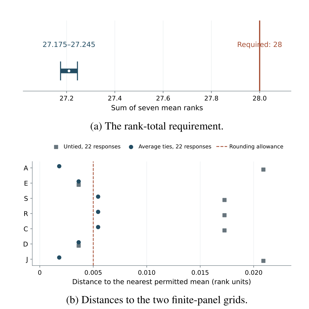
The numerical separation is displayed in Figure 1. The upper panel compares the rounding-compatible total with the required value, while the lower panel displays distances from the two finite-panel arithmetic grids. The large separation between the aggregate interval and 28 explains why printing precision is not an adequate numerical account of the discrepancy. It is also more informative than describing the sum as approximately correct. Rank totals are exact under the complete-ranking interpretation, and the largest allowance justified by rounding has already been included.
The result does not establish that the individual assessments were invalid. Independent item ratings need not sum to 28, and different item denominators may also break the identity for displayed means. Neither possibility can be resolved from the seven values alone. A defensible interpretation therefore has to retain the conditional statement: these aggregates cannot be means of complete rankings within their stated precision. Removing that qualification would turn a mathematical finding into an unsupported assertion about the survey process. Conversely, overlooking the failed identity would permit agreement calculations whose prerequisites have not been established.
The difference between rounding and substantive numerical change remains important throughout the analysis. A radius of 0.005 describes information lost by printing two decimals. A radius large enough to restore feasibility permits changes beyond that information loss. Such changes can be studied to understand decision stability, but they cannot be attributed to respondents without additional records. The feasible sets below are consequently statements about admissible numerical alternatives. They do not express a probability that any particular alternative occurred, and they do not convert an incompatible table into validated panel responses.
B. The stated panel size adds conditional restrictions
The nearest-grid calculations in Table 2 show that five coordinates are incompatible with untied means from 22 equally weighted respondents at the stated precision. Average ties make the necessary grid finer, reducing the number of individually incompatible coordinates to three. SDG alignment, investment return, and internal expertise each remain 0.005455 rank units from the nearest permitted half-integer-total mean, slightly beyond the rounding allowance of 0.005. Their small individual discrepancies are distinct from the much larger collective failure of rank conservation.
| Untied ranks | Average ties | |||
|---|---|---|---|---|
| Code | Nearest mean | Distance | Nearest mean | Distance |
| A | 1.590909 | 0.020909 | 1.568182 | 0.001818 |
| E | 2.136364 | 0.003636 | 2.136364 | 0.003636 |
| S | 3.272727 | 0.017273 | 3.295455 | 0.005455 |
| R | 4.227273 | 0.017273 | 4.204545 | 0.005455 |
| C | 4.727273 | 0.017273 | 4.704545 | 0.005455 |
| D | 5.363636 | 0.003636 | 5.363636 | 0.003636 |
| J | 5.909091 | 0.020909 | 5.931818 | 0.001818 |
A distance at most 0.005 is necessary for compatibility with two-decimal rounding. Coordinate compatibility is not sufficient for a joint ranking matrix.
These calculations should not be used to infer how many experts completed the second round. A change in the effective denominator would change the grids, and unequal weights would remove the simple integer-grid condition. The conservation finding would nevertheless remain for complete assessments under common weights. The two checks therefore answer different questions: the grid examines one stated finite-panel interpretation, while the total examines complete-ranking structure. Agreement between their conclusions strengthens the need for precise reporting, but their assumptions should not be collapsed into a single accusation of numerical error.
The published number of participants is also insufficient to calculate sampling uncertainty. Even if all 22 completed every item, respondent dependence, recruitment, and the distribution of individual positions would remain relevant. Resampling the seven theme means would treat different concerns as interchangeable observational units and would not recover the missing respondent variation. For this reason the analysis reports exact arithmetic and deterministic sensitivity only. The absence of confidence intervals is a consequence of the available information, rather than a decision to conceal uncertainty.
C. The Closest Admissible Continuous Means
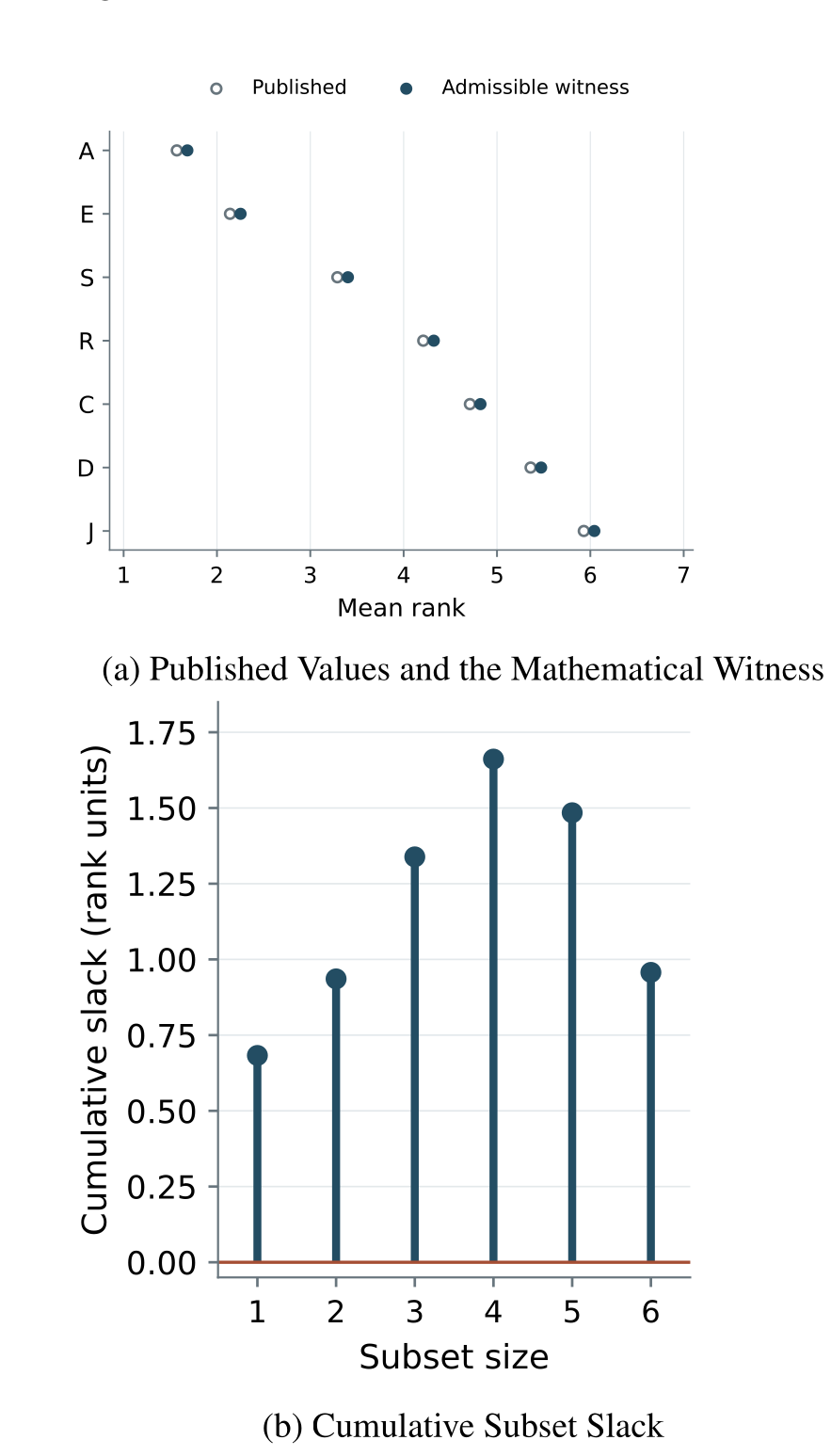
The rank-total deficit is 0.79. Dividing it equally across the seven coordinates gives \(c=79/700\). The resulting vector is
where the displayed entries are rounded and the computation retains the exact rational values. The six cumulative subset slacks are 0.682857, 0.935714, 1.338571, 1.661429, 1.484286, and 0.957143. All are positive, establishing membership in \(\mathcal{P}\). Proposition 1 therefore applies: the minimum displacement is exactly 0.112857 repeating, and the minimizing vector is unique.
The displacement and cumulative checks appear in Figure 2. The uniform shift leaves every difference between two means unchanged. It repairs neither an unknown response process nor an unknown denominator; it simply attains the closest point under the stated distance. The positive cumulative slacks show that no proper subset constraint determines the minimum. Rank conservation is the active restriction. This provides a transparent explanation for the solution instead of presenting an optimization output without its mathematical cause.
Measuring distance from the entire rounding box rather than from its printed centre reduces the required additional displacement to \(0.112857-0.005=0.107857\). This value remains substantially larger than printing uncertainty. The distinction also clarifies how to interpret later thresholds: every displayed \(\delta\) is measured from the printed coordinates, and any allowance explicitly additional to rounding is smaller by 0.005. Neither convention makes \(x^\star\) an observed mean vector. In particular, continuous feasibility does not establish its realizability by exactly 22 equally weighted responses.
An equal displacement should not be understood as equal uncertainty across the themes. It appears here because the selected norm minimizes the largest coordinate change while a fixed total increase is required. If any coordinate were increased by less than the minimizing radius, another would have to increase by more, contradicting minimality. The result is consequently explained by the geometry of the numerical constraint. Its symmetry says nothing about whether access, ethics, or employment was measured more reliably. This interpretation is essential because an apparently balanced adjustment can otherwise acquire an unjustified substantive meaning.
D. Sharp Limits for Pairwise Priority
The full set of pairwise thresholds is shown in Figure 3. All 21 optimization problems attain the half-difference bound in Eq. (8). The smallest threshold is 0.250 for investment return versus internal expertise. A uniform displacement below that value cannot make these two coordinates tie while satisfying the rank constraints. At the threshold, both can equal 4.46 and the remaining coordinates can accommodate the required total. This attainment matters: a distance derived from their difference alone would otherwise remain only a lower bound.
The next threshold, 0.285, is shared by access versus ethical deployment and support for developing economies versus job-loss concerns. Internal expertise versus developing-economy support follows at 0.325. SDG alignment remains strictly ahead of investment return below 0.460, and ethical deployment remains ahead of SDG alignment below 0.575. These different boundaries demonstrate that the seven-item order does not have one uniform degree of numerical stability. Its first loss of strictness occurs in the middle, rather than at the first position.
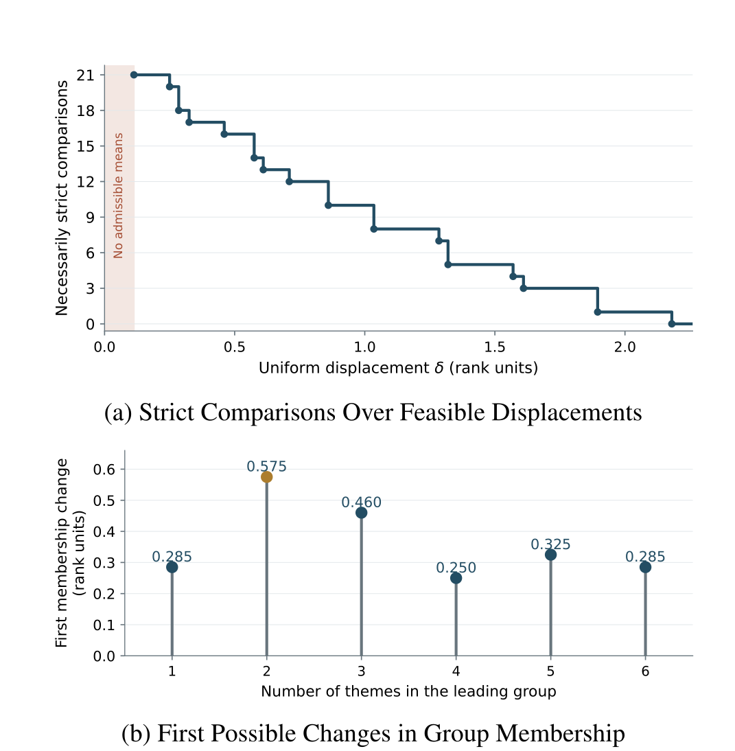
The interval from \(\delta_0\) up to, but excluding, 0.250 contains admissible vectors and preserves all 21 strict comparisons. It is therefore a meaningful range of conditional stability. The empty interval of feasible representations below \(\delta_0\) must not be counted as even stronger evidence. At 0.250 one strict comparison is lost, and at 0.285 two more become non-necessary. The step pattern in Figure 4 records these boundary changes exactly. Values at a threshold are assigned to the side on which a tie is already possible.
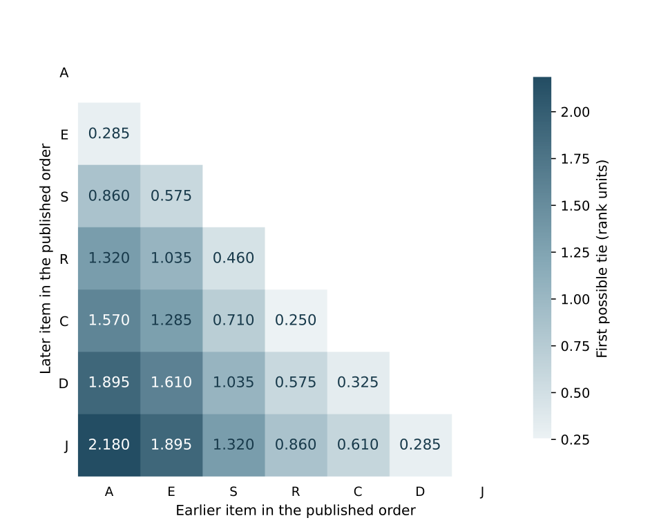
Large pairwise thresholds do not mean that the corresponding policy decision is universally secure. Access versus job-loss concerns has the largest separation radius, 2.180, but the number expresses stability of these aggregate coordinates under this model. It does not establish that employment consequences are small, acceptable, or outweighed by access benefits. Rank separation and substantive trade-offs have different meanings. The numerical evidence can delimit a priority claim while leaving the ethical or operational decision open to information absent from the ranking exercise.
E. Leading Groups Can Outlast Their Internal Order
The leading-group thresholds in Table 3 compare group membership with pairwise order. Access alone remains necessarily first below 0.285. Access and ethical deployment remain the leading two-theme group below 0.575, even though their internal order can fail earlier. Adding SDG alignment reduces the membership threshold to 0.460 because the closest challenger then becomes investment return. A four-theme group is least stable, with its boundary reaching internal expertise at 0.250. The sequence of membership thresholds is consequently not monotone in group size.
| Size | Leading group | Boundary pair | Radius |
|---|---|---|---|
| 1 | A | A–E | 0.285 |
| 2 | A, E | E–S | 0.575 |
| 3 | A, E, S | S–R | 0.460 |
| 4 | A, E, S, R | R–C | 0.250 |
| 5 | A, E, S, R, C | C–D | 0.325 |
| 6 | A, E, S, R, C, D | D–J | 0.285 |
The membership view in Figure 4 makes a practical distinction available without imposing an allocation rule. An organization could identify a group of concerns that warrants early discussion even when an exact sequence within that group is less stable. For the supplied values, access and ethical deployment form the most persistent proper leading group under the uniform displacement convention. That statement concerns the mathematical comparison among the six possible group sizes. It does not prescribe spending proportions or establish that a two-item agenda is sufficient for implementation.
The weakest boundary also identifies a precise information need. If a decision depends on excluding internal expertise while retaining investment return, the fourth-place boundary requires the greatest numerical care. Conversely, a discussion that includes both concerns is not affected by their internal tie alone. This distinction can reduce unnecessary insistence on a fully ordered list. It remains conditional on the ranking representation, and it cannot replace evidence about how the concerns interact within an actual production organization.
F. Mean Priority Does Not Establish Majority Preference
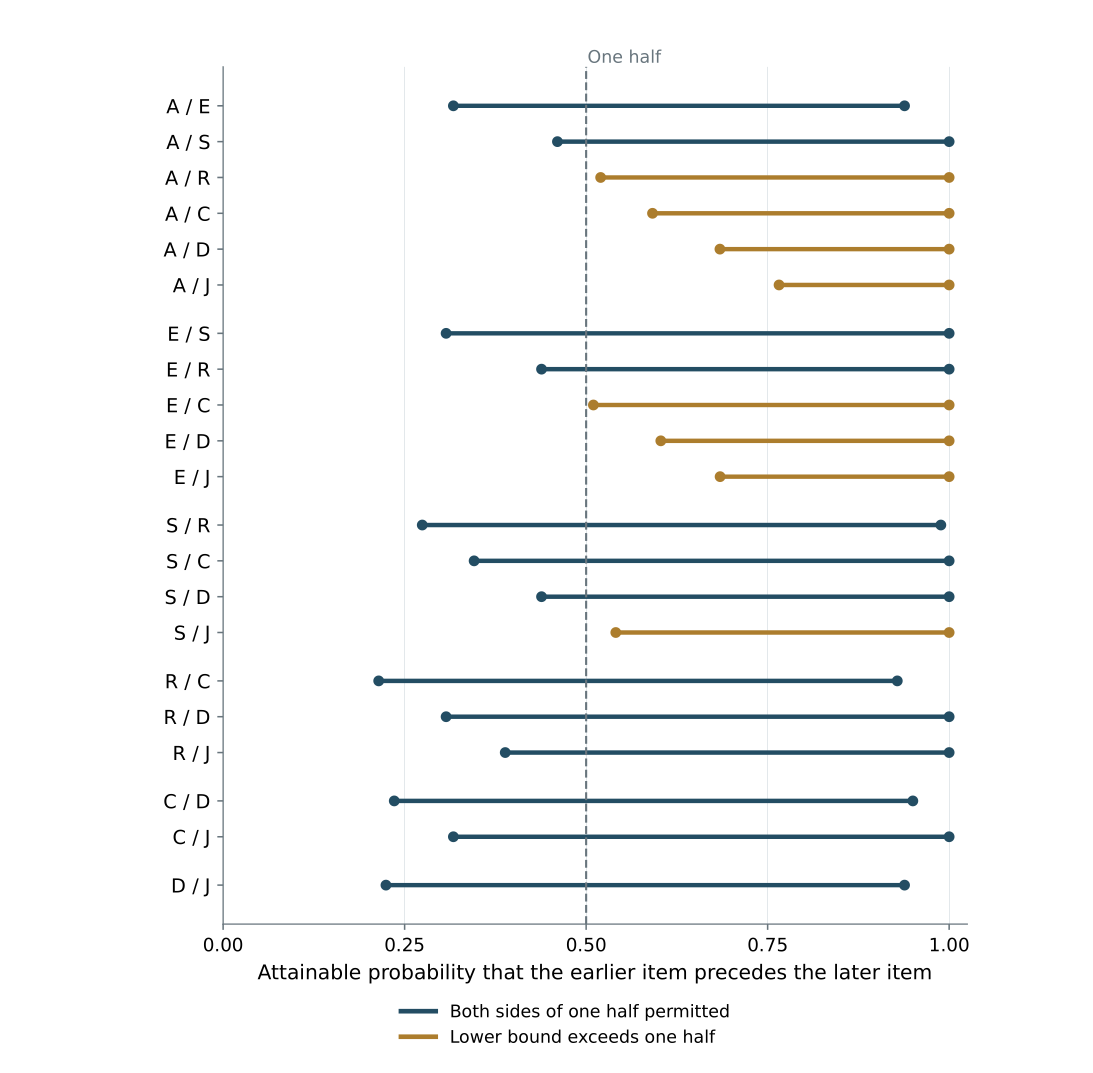
The support intervals in Figure 5 are computed at \(x^\star\) over all complete-ranking distributions satisfying Eq. (10). Access preceding ethical deployment has an attainable probability between 0.317143 and 0.938571. Ethical deployment preceding SDG alignment ranges from 0.307143 to 1.000000. The SDG–investment comparison ranges from 0.274286 to 0.988571. All three intervals cross one half, so the mean vector alone permits either side of the majority boundary for each comparison considered separately.
The same conclusion holds for the remaining adjacent pairs. Investment return preceding internal expertise ranges from \(3/14\) to \(13/14\), or 0.214286 to 0.928571. Internal expertise preceding developing-economy support ranges from 0.235714 to 0.950000, while developing-economy support preceding job-loss concerns ranges from 0.224286 to 0.938571. The six strict mean comparisons therefore do not entail six respondent majorities. A minority assigning large rank differences can affect an average differently from a majority expressing a smaller separation.
The intervals are sharp because each endpoint has a feasible complete-ranking mixture and a matching dual certificate. Their width is not caused by simulation error, incomplete enumeration, or numerical approximation to an unknown probability distribution. It follows from the information discarded by averaging. The 5040 possible rank vectors exhaust the strict-ranking possibilities for seven items. At the same time, the endpoint mixtures are continuous probability distributions and need not correspond to 22 equally weighted respondents. Their values must not be presented as confidence limits for the actual panel.
For every reported endpoint, the accompanying certificate records a feasible distribution and an exact supporting inequality, making the claimed range independently checkable without statistical sampling assumptions.
Some widely separated comparisons do imply a majority within this conditional distribution class. Access preceding job-loss concerns has a lower bound of 0.765714, and access preceding investment return has a lower bound of 0.520000. Across all pairs, eight lower bounds exceed one half. These statements concern the mathematical witness, not the unavailable responses. Moreover, different intervals may attain their endpoints at different mixtures. Reading all lower or upper endpoints as one jointly observed distribution would introduce a further unsupported claim.
The central implication is conceptual as well as numerical. A complete ordering of aggregate means can coexist with substantial ambiguity about individual pairwise preferences. Calling the order a consensus would therefore require a definition of consensus and evidence appropriate to that definition. The present bounds identify precisely which implication fails: adjacent mean priority does not force adjacent majority preference, even after the mean vector is made mathematically admissible under the declared relaxation.
The interval for investment return and internal expertise provides a particularly clear explanation. A probability of one half lies well inside its attainable range, although investment return has the lower mean rank. Both a majority supporting that order and a majority opposing it can be accommodated by complete-ranking distributions with exactly the same seven means. There is no conflict between these findings because a mean difference incorporates how far apart the positions lie, whereas a pairwise majority counts only which item precedes the other. The numerical difference between these summaries is precisely the information that a single ordering conceals.
The complete mean vector supplies information beyond a pairwise difference alone. For access and ethical deployment, Eq. (11) would permit a lower support bound of 0.224286. Requiring the access mean to remain at its witness value raises that bound to 0.317143. Access cannot follow ethics without occupying at least the second position, which limits how frequently that event can occur when its mean position is close to the first. The linear programme incorporates this restriction together with all other mean constraints. For investment return and internal expertise, by contrast, the elementary bounds are already attainable. The distinction explains why some optimized intervals become narrower while others retain their full pairwise width.
G. Concordance Requires a Compatible Numerical Interpretation
The untied concordance expression evaluated at \(x^\star\) is \(0.567934\) to six decimals. This value differs from 0.72, but it is not offered as a replacement estimate for the published coefficient. It belongs to the minimum-distance mathematical witness. The printed aggregates do not satisfy the complete-rank identity required for directly using Eq. (12). It would be equally inappropriate to centre the printed values at their own average, insert the resulting sum of squares into the formula, and label the output a validated panel coefficient.
Ties add a second interpretive restriction. Holding the witness means fixed, obtaining 0.72 algebraically would require a tie correction equal to approximately 21.1203% of the untied denominator. This calculation does not demonstrate that such tied responses exist, particularly for a panel of 22. It states only the denominator change that the equation would require. Establishing attainability would require the actual tie pattern or additional explicit constraints, neither of which is supplied by an item mean and a repeated coefficient.
The distinction between concordance and majority support must also be retained. Without ties, admissible means determine the concordance expression even though they leave many pairwise support fractions undetermined. The wide support intervals therefore do not contradict the diagnostic value of the untied coefficient. They expose a different aspect of information loss. A single global agreement number cannot, by itself, explain which close decisions are vulnerable to reordering or how many experts prefer one particular theme to another.
H. Implications for Manufacturing Governance
The most persistent leading group concerns access and ethical deployment. These themes nevertheless require operational definitions before they can guide an adoption programme. Access may concern the availability of technology, the ability of employees to use it, or the capacity of smaller organizations to participate. Ethical deployment may concern accountability, discrimination, or the treatment of affected people. Jobin and colleagues document common ethical principles alongside differences in how AI guidance expresses them, while Mehrabi and colleagues examine distinct sources and definitions of algorithmic unfairness [35], [36]. Their work supports specifying the obligation at issue rather than treating an ethics rank as evidence that the obligation has been fulfilled.
Organizational procedures also matter. Raji and colleagues describe internal algorithmic auditing, and Rakova and colleagues examine how organizational conditions enable or obstruct responsible AI practice [37], [38]. These contributions make a connection between governance aspirations and accountable work. In the present analysis, a stable place for ethical deployment can justify preserving it as a topic of deliberation. The rank itself cannot establish that responsibilities have been assigned, that a review process has been followed, or that affected workers can challenge a decision. Those are separate organizational observations.
Investment return and internal expertise form the first vulnerable pair. Treating their order as a rigid sequence would overlook the possibility that capability development is part of producing an economic return. The automation–augmentation analysis of Raisch and Krakowski examines tensions between substituting for and complementing human work, while Kellogg and colleagues analyse organizational control associated with algorithms [39], [40]. These accounts motivate examining who exercises judgement and how work changes. They do not establish a particular causal relationship among the seven themes. The numerical result supports caution about separating the middle priorities, not a new claim about their effects.
Manufacturers can therefore distinguish a stable discussion agenda from an evidence-based investment calculation. The former may use the leading-group results, with their conditions stated. The latter requires costs, expected operational consequences, dependencies between activities, and an explicit decision objective. Similarly, SDG alignment requires an identified environmental or social outcome rather than a place in an ordering. The present calculations do not convert priorities into monetary weights or presume that the distance between two rank means measures the magnitude of their industrial benefits.
The employment item illustrates an additional boundary of interpretation. Its final position is an ordering among the seven supplied concerns, not a threshold below which employment consequences may be disregarded. Concern frequency, anticipated severity, distribution of consequences, and available forms of participation could all matter to a workplace decision. None is measured by the published mean. The mathematically stable comparison between access and employment therefore cannot justify dismissing worker involvement. It establishes separation between aggregate coordinates while leaving the content and procedural obligations of a particular implementation to be assessed on their own evidence.
I. Scope and Limits of the Conclusions
The empirical scope remains one set of seven aggregate assessments. It does not support comparisons between sectors, countries, plant sizes, or technology families. The themes are heterogeneous, and their labels do not specify a common intervention scale. A preference for addressing access before another concern cannot be interpreted as a measured substitution rate between two projects. The method addresses the consistency and stability of numerical priorities within these limitations, rather than overcoming them through added assumptions about manufacturing behaviour.
The uniform distance convention is transparent but not substantively privileged. Different item-specific tolerances or a different distance could change the nearest admissible vector and some separation limits. The current results are exact for the stated convention, which treats every printed coordinate in rank units. No claim is made that the selected radius represents the actual amount or distribution of reporting error. A decision maker can inspect the full threshold schedule without being told that one unexplained tolerance is the correct industrial choice.
Finally, the analysis cannot resolve whether the displayed values arose from ratings, complete ranks, incomplete responses, or a transformation that was not numerically specified. The appropriate conclusion is correspondingly bounded. Complete-rank interpretation fails at printed precision; conditional stability can still be characterized beyond the minimum feasible displacement; individual preferences remain only partially identified in the explicit continuous calculation. None of these statements requires fabricated observations. Their value lies in preventing the numerical precision of an aggregate table from being mistaken for information that the table does not contain.
The information needed to narrow these conclusions is specific. A complete response matrix with identifiers removed would establish the joint rankings, reveal tied blocks, and permit verification of the displayed means and concordance. If item ratings were used, the response categories and transformation rule would instead establish the appropriate interpretation. Item-level completion counts would distinguish a common denominator from differing respondent subsets. Such information would address the identified numerical ambiguity directly. More decimal places, a larger bibliography, or an additional conceptual illustration would not resolve it without clarifying how the assessments were obtained and combined.
V. Conclusion
The research question concerns which manufacturing AI priorities remain defensible when seven rounded summaries are required to represent complete rankings. At their printed precision, none has a jointly admissible complete-rank representation: the largest rounding-compatible total is 27.245 rather than 28. This conclusion is independent of panel size and survives average ties. Conditional analysis becomes possible only after admitting a uniform displacement of at least \(79/700\) rank units from the printed values. That minimum identifies a numerical distance, not the unobserved expert assessments.
Within the stated continuous rank model, every strict comparison persists from that minimum up to 0.250. Investment return versus internal expertise is the first comparison to permit a tie. Access and ethical deployment retain their joint position as the leading two-theme group below 0.575, although their internal order can fail at 0.285. These results answer the ordering question with explicit boundaries. They support a distinction between selecting a leading group for attention and asserting a fully resolved sequence of concerns.
The agreement question has a different answer. At the minimum-distance admissible vector, each adjacent comparison admits complete-ranking distributions on both sides of the majority boundary. Aggregate order therefore cannot establish adjacent majority preference. Untied concordance has a computable diagnostic expression at valid means, but interpreting the displayed coefficient requires compatible rank summaries and the appropriate tie information. The defensible contribution is thus a precise account of what the published priority numbers permit one to conclude. It establishes neither a new industrial performance result nor a recovered expert panel, and it leaves the practical allocation of manufacturing resources dependent on evidence about the activities actually being considered.
Funding
This research received no specific grant from any funding agency in the public, commercial, or not-for-profit sectors.
Data Availability
The data analysed in this study were obtained from published sources cited in the manuscript. The data and analytical procedures required to reproduce the reported results are provided within the article and its supplementary materials, where applicable.
Conflicts of Interest
The author declares no conflicts of interest related to this work.
Declaration of Generative AI Use
Generative artificial intelligence was used solely to assist with language editing and improve the clarity of the manuscript. The author reviewed and revised all AI-assisted text and assumes full responsibility for the accuracy, originality, integrity, and final content of the article.