
People increasingly seek to satisfy higher-level cultural and artistic needs after meeting basic requirements such as clothing, food, housing, and transportation. Learning to play the piano has consequently become an attractive activity for many people. In recent years, interest in piano learning has reportedly increased substantially among learners of different ages, with young children representing a particularly important group of students. In some urban middle-income and higher-income families, it has been claimed that one in five households has parents who want their children to learn the piano and that applications for piano grade examinations have increased by approximately 20% each year. Such figures are highly dependent on the particular population and educational system being considered, and their interpretation requires reliable information about the surveyed households, geographical location, and reporting period. Moreover, reforms in the national education system and the expansion of educational provision have reportedly increased the demand for piano instructors. In the field of piano education, professionally qualified teachers are sometimes described as a scarce resource, and such shortages may not be easily resolved within a short period of time.
Piano education can also be expensive, with some accounts suggesting that an average piano costs at least $10,000. Piano instruction is often delivered through individual, one-to-one lessons, and tuition fees have been reported as ranging between $100 and $400 per lesson. These estimated costs can differ considerably by instrument type, country, teaching institution, and period, and published comparisons of piano education therefore require a carefully defined market and a consistent pricing basis. In this situation, some students attend only one formal piano lesson per week and must undertake much of their remaining practice independently. Without sufficient guidance, learners may develop inefficient practice habits, encounter avoidable difficulties, and progress at a slower rate than expected. Independent practice and the development of supportive learning technologies have therefore attracted attention in research on piano education [1], [2]. Access to piano instruction may also be restricted by geographical distance, scheduling difficulties, and the limited availability of qualified teachers, which can discourage interested learners from continuing their studies. Studies of asynchronous lessons and comparisons of on-site and distance instruction offer relevant evidence about the possibilities and limitations of remote teaching [3], [4].
Excessive or unnecessary movement is a common technical difficulty encountered during piano training. Pianists may need to reduce avoidable external force, simplify their playing movements, and improve finger stability in order to produce a focused, powerful, and bright tone. To maintain a consistent tone throughout a passage, it is useful to avoid unnecessary vertical wrist movement, pay particular attention to octave passages, and minimize excessive movement during rapid playing. These adjustments can help performers achieve smoother and more coordinated motion. Biomechanical studies comparing experienced and novice pianists, investigating tactile feedback, and examining the influence of trunk motion and touch provide a research basis for considering movement organization and control, although they do not establish a universal prescription for every performer [5]–[7]. After each note is sounded, the hand should be prepared to release the key and transfer the required movement to the next note, particularly during rapid groups of notes. The transfer of movement and effort between the fingers should remain as relaxed and efficient as possible. It is also important to avoid consciously applying excessive pressure through the wrist. This helps the weight and movement of the hand remain coordinated with the movements of the fingertips. For a smooth and even tone, the pianist’s arm, elbow, and wrist should move in a manner that supports the intended fingertip action.
In addition, tonal production is affected by the support and coordination of the fingers. Effective finger support is an important element of piano technique because it influences both mechanical control and the resulting quality of sound. Mr. Ling Zhuping has stated that the supporting capacity of the fingers is limited and that excessive pressure from the arm may contribute to discomfort or injury in the hand muscles. Nevertheless, the fingers should not be placed loosely on the keys without appropriate contact or control, because insufficient finger support may also weaken the intended tonal effect. In the climax of the fourth variation of Glinka’s “The Nightingale,” for example, the left hand plays a leaping eighth-note broken-chord figure while the right hand performs a sixteenth-note broken-chord figure in octaves, requiring considerable coordination and finger stability. The fingers should maintain secure but moderate contact with the keys rather than exerting excessive pressure, which may restrict finger flexibility; meanwhile, the palms should remain relaxed instead of tense. Because the five fingers differ in their anatomical characteristics and mechanical capacities, coordinated and even finger control may require additional practice, particularly for the little finger. When each finger can provide independent support, the hands maintain an appropriate level of relaxation, and movement is transferred smoothly from the arms toward the keys, the pianist is better positioned to coordinate tonal quality and loudness. It is also important to maintain a sense of support between the shoulder and the fingertips during performance. Although the centre of the palm may remain slightly arched, the hand as a whole continues to contribute to controlled support. Across different tonal demands and playing speeds, stable finger positioning and controlled movement can help performers retain the necessary mechanical support. These considerations demonstrate the importance of finger stability, coordination, and support in the performance of piano works. Research on piano biomechanics and historical approaches to touch supports their pedagogical relevance, while suggesting that instructions about hand position should be adapted to the individual performer and the musical task [7], [8].
In piano performance, the manner in which the keys are touched can influence the perceived quality of the tone and the range of expressive variations available to the pianist. If touch is poorly controlled, the tonal result may be unsatisfactory, and the variety of expressive effects can be restricted. The piano is a complex instrument whose performance requires not only technical competence but also a thorough understanding of the musical work and an ability to convey its intended ideas and emotions. Studies of piano pedagogy and timbral perception have highlighted the importance of coordinating touch, auditory perception, and musicians’ embodied understanding of sound [8]–[10]. The relationship between a pianist’s description of timbre and acoustically measurable changes remains an important distinction, and educational discussion should not treat every perceived tonal difference as proof of an independently altered acoustic spectrum. The piano is capable of producing a wide range of dynamic effects, and appropriate key-touch techniques are important for performing different levels of tonal intensity. Tonal production is influenced by fingertip movement, the stability of the hand, and the flexibility and relative independence of the fingers. Accordingly, carefully developed touch technique is a central aspect of effective piano performance. Digital interfaces and interactive learning technologies have also been investigated as possible supports for piano education, providing a wider context for the sensor-based methods discussed in the following sections [1], [2], [11]. These published applications establish the feasibility of studying instructional technologies; they do not, by themselves, establish that the particular system described in the present manuscript improves students’ performance.
To explore the relationship between piano touch technique and tonal expressiveness, the playing function must first be analysed. The overall analytical procedure is presented in the block diagram shown in Figure 1.
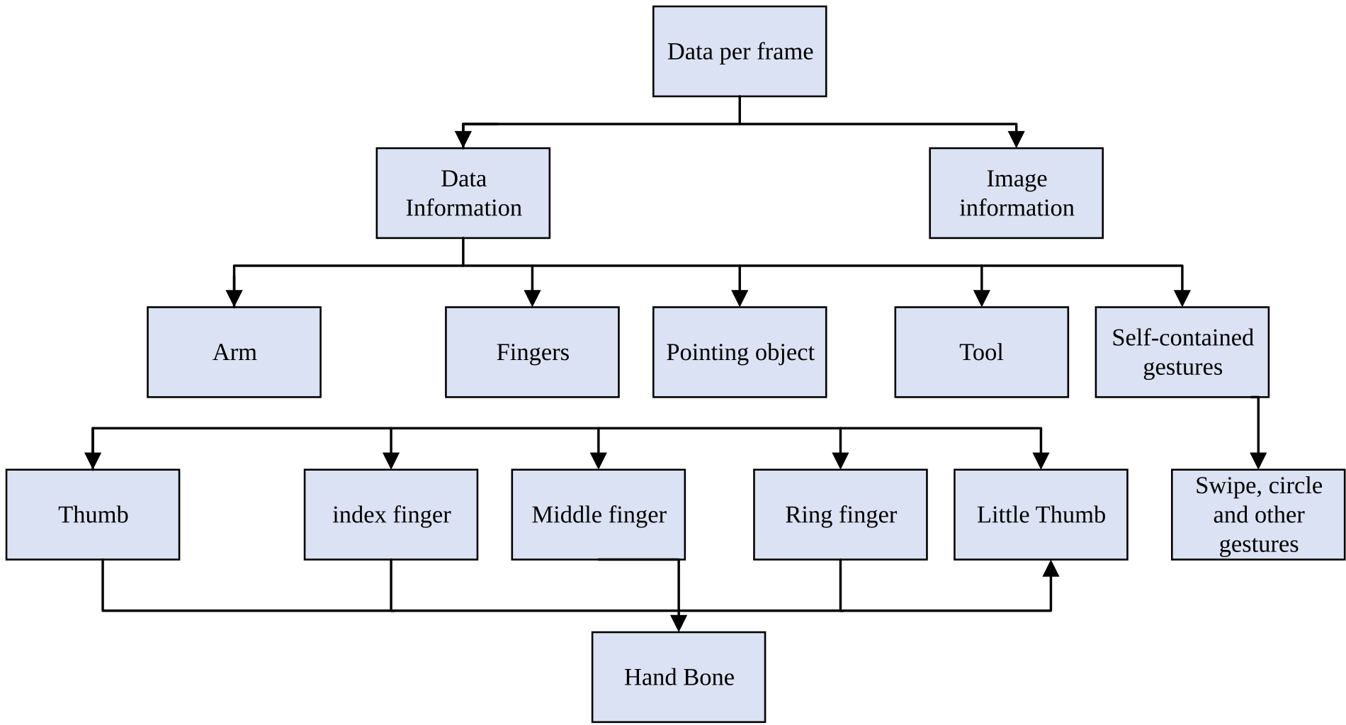
When an object tracked by the Hand Controller is processed through the onFrame() callback function, the system obtains data frames representing individual parts of the tracked object. The structure of the resulting data frame is illustrated in Figure 2.
High-accuracy tracking of finger positions can produce high-frequency noise during gesture detection, because both small involuntary finger tremors and fluctuations in the sensor measurements may affect the recorded coordinates. Consequently, filtering and smoothing procedures are required to reduce unwanted fluctuations in the recorded motion data. Published evaluations of the Leap Motion Controller document measurement accuracy and reliability limitations, including differences between static and dynamic tracking conditions [12], [13].
The trajectory followed by a moving finger can be approximated by a continuous curve. Accordingly, the relationship between the finger’s coordinate position and time can be expressed using the following functions.
Taking the first-order derivatives of the coordinate functions in Eq. (1) gives the following expressions:
Eq. (2) describes the rate of finger movement along the indicated \(Z\) and \(J\) axes, from which the angle associated with the direction of finger movement can be determined.

Because the recorded discrete observations are collected at fixed, equal time intervals, and because these sampling intervals are relatively short, the derivatives in Eq. (2) can be approximated using differences between adjacent observations. The direction of finger motion can therefore be calculated using the following expression.
The angular change in the direction of the recorded movement between two consecutive sampling points can consequently be expressed using Eq. (4).
A threshold, \(\tau\), is then applied to identify possible jitter in the movement data. When the angular change remains below the selected threshold, the observation is retained; when the angular change exceeds the threshold, the observation is treated as potential jitter noise and filtered out, according to the following decision rule.
According to the repeated experiments described in this study, the threshold in Eq. (5) was set at 30 degrees. In particular, changes in the direction of a movement gesture were retained when their angular magnitude was less than 30 degrees, whereas observations with an angular change greater than 30 degrees were removed during the initial filtering stage.
To suppress remaining high-frequency noise more effectively, the simple moving average (SMA) filter can additionally be applied as a data-smoothing technique. The operation of this filter is represented by the following equation.
In Eq. (6), \(S\) represents the calculated moving-average value of the data, while \(n\) denotes the number of observations included in the averaging window. The choice of \(n\) affects the overall smoothing result: an excessively large window may remove meaningful details of the movement gesture, whereas an excessively small window may fail to suppress unwanted fluctuations adequately.
Hidden Markov models (HMMs) are probabilistic models that can be applied to sequential classification and labelling problems. They have been employed in several fields, including speech recognition, natural language processing (NLP), bioinformatics, pattern recognition, and artificial intelligence. Their ability to describe sequences of hidden states and observable events also makes them relevant to the analysis of time-dependent motion data. Established treatments explain both HMM inference and its relationship to statistical pattern-recognition methods [14], [15].
The HMM is represented by the following model parameters and expressions:
In addition to the three principal elements specified above, applying an HMM to observed data involves addressing both the parameter-learning problem and the sequence-prediction problem. These tasks must be distinguished because they describe different stages of model estimation and interpretation.
The expression for the output probability associated with the state sequence \(Q=q_1,q_2,\ldots,q_r\) under the specified hidden Markov model \(\lambda\) is given as follows.
The probability expression for generating the observed sequence, conditional on the underlying state sequence, is presented below.
Using the expressions above, the observation probability for a given model \(\lambda\) can be written in the following form.
The expression in Eq. (10) is intended to account for the possible hidden-state sequences associated with the observed sequence \(O\). The direct calculation is described as having approximate computational complexity \(2TN^T\), whereas the corresponding dynamic-programming approach is described as having complexity \(N^2T\). These complexity expressions depend on the definitions of the numbers of observations, states, and transitions and should be checked against the implemented model. This comparison is presented as part of the computational motivation for using sequential models in the proposed gesture-recognition procedure.
(1) Forward algorithm
Given a model \(\lambda\), the forward probability is defined as the probability of observing the partial sequence \(o_1,o_2,\ldots,o_r\) up to time \(t\) and reaching the specified state \(q_i\) at that time. This probability is expressed in the following form.
(2) Backward algorithm
Given a model \(\lambda\), the backward probability describes the probability of the future observations \(o_{t+1},o_{t+2},\ldots,o_T\), conditional on the state at time \(t\) being \(q_i\). The corresponding probability expression is presented below.
The relationship between the forward and backward probabilities is shown in Figure 3.

When the available training data consist only of observation sequences, HMM parameters can be estimated using the expectation-maximization (EM) algorithm, which is a standard approach to unsupervised parameter learning in probabilistic sequential models. The general estimation principle is established in foundational work on maximum-likelihood estimation from incomplete data [16]. For the hidden Markov model, let \(O=(o_1,\ldots,o_T)\) denote the observed sequence, \(I=(i_1,\ldots,i_T)\) denote a possible hidden-state sequence, \(\lambda=(A,B,\pi)\) denote the model parameters to be estimated, and \(\bar{\lambda}\) denote the current parameter estimates. Following the HMM auxiliary-function formulation [14], [16], the unnormalized EM objective can be written as
The terms \(a_{ij}\) and \(b_j(o_t)\) represent the state-transition and observation-emission probabilities, respectively. The objective in Eq. (13) uses the joint probability \(P(O,I\mid\bar{\lambda})\) as a weight; dividing by the fixed quantity \(P(O\mid\bar{\lambda})\) gives the conventional normalized conditional-expectation objective and does not change its maximizing parameter values.
(1) To estimate the initial-state probability \(\pi_i\), the first term in Eq. (13) can be collected by initial hidden state as follows:
The parameter \(\pi_i\) must satisfy the normalization constraint \(\sum\limits_{i=1}^{N}\pi_i=1\). Therefore, the Lagrange multiplier method can be applied to construct an appropriate constrained objective function and derive the required parameter estimate.
Taking the partial derivative of the constrained objective function and setting the resulting expression equal to zero gives the following condition:
Solving the resulting condition yields the following estimate for the parameter \(\pi_i\):
To estimate the observation-emission parameters \(B\), the third term in Eq. (13) can be reorganized by hidden state and observation time as follows:
The Lagrange multiplier method is again applied, this time with the constraint \(\sum\limits_{k=1}^{M}b_j(k)=1\). The partial derivative of \(b_j(o_t)\) with respect to \(b_j(k)\) is nonzero only when the observation \(o_t\) is equal to \(v_k\), which is the corresponding discrete observation symbol.
First, consider the manual evaluation of musical performance. Its principal elements include the performance environment, the performer, the musical instrument, and the listener. The listener’s perception of the resulting music forms an important component of the evaluation process. Using every individual tonal characteristic as an input parameter may be impractical because several features contain redundant information concerning the factors that influence performance quality. The principal characteristics of a musical tone include pitch, intensity, duration, and timbre. If timbre is excluded from the immediate analysis, the remaining characteristics can be obtained from messages generated by a MIDI instrument. Representing pitch, onset, duration, and expressive timing as computational features is consistent with established approaches to music-information processing [17]. Duration-related features are associated with the beat and rhythm, while the present example focuses on the synthesis and evaluation of pitch characteristics.
The pitch properties obtained from the piano’s MIDI messages are represented using 127 discrete levels. A difference of one level represents a semitone, corresponding to adjacent notes on the piano keyboard without distinguishing between black and white keys. Playing an incorrect key produces a pitch error that may have a substantial effect on the musical result. Consequently, a pitch deviation is classified as an error regardless of the size of the difference. The combined evaluation factor for each measure is therefore determined by quantifying the number of incorrect keystrokes.
The MIDI note numbers in the source draft are given as 71, 7l, 72, and 74 for the example pitches B, B, C, and D. The second code contains a possible transcription error (the letter “l rather than the numeral “1) and should be confirmed using the original MIDI record. If all four notes are played correctly, the input parameter is \(4/4=1\); if only three notes are played correctly, the corresponding parameter is \(3/4=0.75\), and the same calculation is extended to other outcomes. MIDI messages also provide a discrete measure of note-on velocity associated with performance intensity. The coding of intensity depends on the precise MIDI message definition, the interpretation of note-on velocity, and the device-specific treatment of zero velocity, all of which should be specified for a reproducible analysis. To establish a reference level for intensity, the performance of a musician with a strong command of the beat, such as an experienced piano teacher, can be used to obtain standard measurements of dynamic intensity. For example, in the first measure of “Ode to Joy,” the reference intensity values are 100, 70, 90, and 70, representing the intended dynamic pattern. If a performer produces the corresponding values 98, 75, 80, and 70, the total absolute intensity deviation for that measure is \(2+5+10+0=17\). For a musical passage containing 16 measures, the proposed representation consequently requires 16 input-layer elements in the neural network, with one element associated with each measure.
The pitch, intensity, and duration of each chord are evaluated using the method described above, with the observed values compared against the corresponding reference values. The difference in pitch is determined by first identifying whether the fundamental note of the chord has been played correctly and then examining any remaining deviations.
An example illustrating the effect of SMA smoothing is provided in Figure 4. Figure 4(a) presents the original three-dimensional combined-velocity data recorded during a finger-click action, whereas Figure 4(b) shows the corresponding data after filtering.
During gesture acquisition, the Leap Motion device records movements over a period of time and may capture multiple consecutive gestures. These recordings contain long sequences of discrete observations representing different stages of movement. As a result, it is necessary to segment the continuous data and extract individual gestures before performing subsequent gesture classification and recognition. Research on Leap Motion-based gesture recognition demonstrates how tracked fingertip positions and orientations can be transformed into features for classification [18].
A sliding-window segmentation technique is used in this study to isolate individual gesture movements. The technique extracts a fixed-length window from a continuous sequence of motion signals, moves that window along the time axis, and calculates the average velocity of observations within each window. When the average velocity falls below a selected threshold, the corresponding window is interpreted as containing no significant gesture movement. Conversely, when the average velocity reaches a sufficiently high value, the window is treated as containing gesture activity. The chosen window can then be positioned to cover the interval associated with an individual gesture movement.

The instantaneous combined velocity of the fingertips and the average combined velocity over the selected window are calculated using the following expression:
Here, \(V_i\) denotes the three-dimensional instantaneous combined velocity of the \(i\)th sampled point. Because the sampling interval between adjacent observations is fixed, the calculation adopts \(\Delta t=1\) for the discrete-time representation. The parameter \(k\) denotes the width of the sliding window. The Leap Motion sampling rate is stated as 100 frames per second, and typical gesture movements are assumed to last no longer than one second; consequently, the window width is set to \(k=100\) observations. The minimum gap threshold is set to 1, and any window whose average combined velocity falls below this threshold is treated as containing no detectable gesture movement.
Figure 5 illustrates the segmentation and extraction of individual finger-click actions. The example indicates that the sliding-window technique can identify the time intervals associated with successive clicks, thereby allowing individual movements to be isolated for subsequent recognition. This segmentation stage provides the data structure needed for the next steps in gesture classification and motion analysis.

Each individual gesture extracted during the preceding stage contains 100 sample points, with each point recording coordinate information along the \(x\), \(y\), and \(z\) axes. To facilitate HMM-based modelling, the complete gesture is divided into smaller frames, and characteristic features are extracted from each frame. These features are subsequently encoded according to the direction of movement velocity. In this way, each gesture can be represented as a sequence of simpler component actions, or meta-actions, whose feature vectors form an ordered sequence of observations. The original gesture is therefore represented as an \(n\)-dimensional, time-dependent feature vector. Frame-based decomposition is intended to reduce the dimensionality of the recorded data while preserving the movement characteristics that are most relevant for recognising the gesture.
The direction of finger velocity is treated as an important descriptor of each gesture’s characteristic movement. Accordingly, the normalized combined-velocity vector is calculated before directional encoding is performed. The transformation between spherical coordinates and the Cartesian coordinate system is described using the angles \(\theta\) and \(\varphi\), measured with respect to the indicated \(z\) and \(x\) axes. This geometric representation is illustrated in Figure 6.
As shown in Table 1, the velocity-direction vector is quantized into 26 coding levels on the basis of the angles \(\theta\) and \(\varphi\). First, the polar angle \(\theta\) is divided into segments separated by 45 degrees. For directions away from the \(z\) axis, the \(xy\) plane is then divided into eight equal angular sectors, with each sector receiving a distinct code, as illustrated in Figure 7. The special cases \(\theta=0^{\circ}\) and \(\theta=180^{\circ}\) each receive a single code. This procedure produces a total of \(3\times8+2=26\) directional codes.

| \(\theta\) value range | Coding segment |
|---|---|
| \(0^\circ\pm22.5^\circ\) | 0 |
| \(45^\circ\pm22.5^\circ\) | 1-8 |
| \(90^\circ\pm22.5^\circ\) | 9-16 |
| \(135^\circ\pm22.5^\circ\) | 17-24 |
| \(180^\circ\pm22.5^\circ\) | 25 |

For each subframe of a recorded gesture, the mean values of the angles \(\theta\) and \(\varphi\) are calculated from the normalized combined-velocity vectors belonging to that subframe. The resulting mean direction is then encoded using the quantization levels specified in Table 1.
The artistic style, melodic development, and structural organization of a piano performance provide important contexts for understanding tonal expression. Therefore, a detailed analysis of piano tone should consider the techniques used to touch individual keys, the sequence in which those keys are played, and the intensity of the keystrokes as the melody and musical texture change. Such an approach may help performers develop more deliberate control over tonal production and improve the expressive quality and musical impact of their playing. Different key-touch methods can produce noticeably different performance outcomes, depending on the musical passage and the intended expressive effect. The relationship between the musical image and its mode of expression, together with the performer’s ability to select and coordinate suitable key-touch techniques, can contribute to improvements in technical execution, artistic presentation, emotional communication, and the overall interpretation of a piano composition. The analytical framework discussed in this paper emphasizes the role of detailed movement characteristics in understanding finger gestures and their possible relationship to performance technique. The material presented does not provide a controlled comparison of student learning outcomes, classification accuracy, or measured improvements in tonal expression; those educational and technical outcomes would require a separately documented evaluation.
The authors contributed equally.
The authors declare no conflicts of interest.
Data are available from the corresponding author upon reasonable request.
No funding was received for this study.