
I. Introduction
Choosing how to repair a generated program is a decision about losses as well as gains. A configuration can have the highest average test fraction while failing on a task for which another configuration preserves substantially more correct behavior. Such a result does not invalidate the favorable average, but it changes the question that the average can answer. Automated algorithm selection studies complementary strengths across problem instances and emphasizes that the preferred algorithm depends on the instance distribution and performance objective [1]. Genetic code repair provides a clear setting for this distinction because both the fitness function and the mechanism selecting parents can change the direction of an observed effect.
Research on automated repair of programs produced by language models establishes the relevance of executing and modifying generated code rather than accepting its textual plausibility [2]. Work with large pretrained models also demonstrates that repair outcomes depend on how candidate changes are elicited and evaluated [3]. These contributions concern the production of candidate programs. The present study concerns a subsequent decision: choosing among specified genetic configurations when their published outcomes are heterogeneous. A configuration is treated as an available action, and the decision is evaluated against the other actions on the same task and model. This formulation preserves the distinction between creating a better repair algorithm and deciding how existing alternatives should be used.
Feedback has different roles in different repair systems. Conversational repair uses execution information to guide additional language-model responses [4], whereas CodeT uses generated tests and execution agreement to select among candidate solutions [5]. Neither mechanism is equivalent to changing a fitness function inside an evolutionary population. Evaluations of self-repair further show that apparent gains depend on the quality of feedback and on accounting for the cost of obtaining it [6]. Research on intrinsic reasoning correction addresses the narrower setting without external feedback [7]. Its conclusions therefore cannot be transferred directly to a repair procedure receiving explicit input–output tests. These distinctions motivate a comparison restricted to four configurations sharing the same published genetic-search setting.
The quality of evaluation also determines what a repair score means. Stronger tests can expose incorrect programs that pass a smaller test collection, as demonstrated by rigorous evaluation of code generated by language models [8]. Repository-level issue resolution, represented by SWE-bench, additionally involves dependencies and coordinated modifications across files [9]. LiveCodeBench emphasizes evolving task collections and the timing of model evaluation [10]. These resources establish important boundaries for interpreting compact program-synthesis tasks. A median fraction of passed cases is evidence about behavior on a stated test set; it is not a proof of functional correctness or an estimate of success across arbitrary repositories.
Genetic improvement modifies existing software using search guided by specified objectives [11]. Within that tradition, changing the way candidate programs are ranked can alter which partial solutions remain available for later variation. Count fitness prioritizes the number of cases passed. A discrepancy term distinguishes programs tied on that count according to the distance between returned and expected values. Tournament selection compares aggregate rankings within sampled groups, while lexicase selection considers cases separately. These choices describe different information pathways through the search. Their combined effect need not equal the sum of the changes obtained by introducing each choice separately.
The selection literature provides reasons to examine this dependence without presuming its direction. Epsilon-lexicase selection was developed to adapt casewise selection to continuous error spaces [12]. Random subsampling can improve lexicase performance under specified evaluation budgets [13]. Detailed investigation of down-sampled lexicase attributes its principal advantage to examining more candidate individuals within a computational budget, rather than establishing a universal reduction of overfitting [14]. Further work shows that the benefits of down-sampling vary with the selection procedure [15], and comparative analyses investigate its behavior across program-synthesis settings [16]. Consequently, a positive combined result cannot by itself identify a universal mechanism or an independent contribution from either component.
Configuration analysis elsewhere in machine learning makes a related distinction. Functional analysis of variance can quantify how hyperparameters and their interactions contribute to performance variation [17]. Analyses across datasets reveal that parameter importance depends on the collection of problems being considered [18]. The four-configuration design examined here does not require fitting a surrogate model over a large parameter space. It permits a direct difference of differences within every eligible task–model pair. That calculation is simpler than a global importance model, but its interpretation still depends on the level of aggregation: a contrast of medians is not automatically a median individual-run effect.
Algorithm selection has developed practical responses to complementary performance. SATzilla predicts which solver is suitable for a problem instance [19], while AutoFolio configures an algorithm-selection procedure itself [20]. ASlib provides a common representation for algorithm outcomes and instance information [21]. Broader accounts distinguish selection, scheduling, and portfolio construction [22]. These precedents clarify the role of information available before a decision. A selector based on task features is a different object from a retrospective rule that chooses the largest reported outcome in each row. The latter is useful for measuring opportunity loss, but it cannot be presented as a deployable policy with advance knowledge of test outcomes.
Minimax regret offers a decision criterion when the loss from choosing a less favorable action matters more than its average across the observed collection. Earlier work formalizes this criterion under incomplete utility information [23]. Robust optimization represents uncertain quantities through specified sets [24], and practical guidance stresses that the shape of these sets must match the information actually available [25]. Here the uncertainty set is limited: it records the display precision of published fractions. It does not represent an estimated distribution of random seeds, future tasks, or program outputs. Distributionally robust optimization treats ambiguity about probability distributions [26]; that richer interpretation would require information absent from the present record.
The choice of observational unit also determines the scope of originality. A configuration-level dataset can be constructed by reorganizing documented outcomes and calculating quantities absent from the published tables, while retaining the same empirical provenance. Its contribution lies in the question and calculation, not in claiming that the underlying programs were generated again. This distinction is especially relevant when published summaries are sufficiently complete for an exact decision calculation but insufficient for estimating execution-level variability. The present four-action utility matrix permits the former analysis. It cannot support claims about independently sampled programs, previously unobserved defects, or newly measured repair rates.
The research question is therefore: how should a genetic code-repair configuration be chosen when fitness and selection interact and only rounded median test fractions are available? The analysis answers this question at the level of the finite published collection. It examines the four-cell interactions, checks which signs survive rounding, compares fixed choices with randomized choices over median-score utilities, and evaluates sensitivity to removing whole tasks. The contribution is an auditable connection between nonadditive configuration outcomes and a decision rule with an explicit loss criterion. It does not introduce another repair operator or claim additional executions of the language models.
II. Materials and Methodology
A. Numerical Material and Unit of Analysis
The numerical material comprises the genetic-improvement [27]. These tables are credited for every input median; the accompanying cell-level file records its table number, page, task, model, configuration, and printed token. Appendix comparison Tables 7–9 provide repeated entries for transcription checks and are not counted as additional observations. The complete record describes 25 PSB2 tasks and four historical generator labels. The present analytical dataset contains the four configuration outcomes for every pair with numerical entries under all four conditions, together with calculated contrasts and decision losses.
The PSB2 collection was designed for general program synthesis with varied task specifications [28]. Its task universe gives 100 possible task–model combinations. Fifty-six combinations were omitted from genetic repair after at least one of ten initial generations satisfied the training cases. Of the 44 remaining combinations, CodeLLaMA 7B with Solve Boolean was marked unparseable under the grammar. Excluding that combination leaves 43 complete pairs across 18 task names. CodeLLaMA 7B (CL7) contributes 15 pairs, LLaMA 3 8B (L3) contributes 12, and ChatGPT (CG) and GPT-4 (G4) contribute eight each. These counts are conditional on the initial-generation screening rule and do not constitute a comparison of overall model capability.
The historical model labels must also remain separate from present product names. Their recorded outcomes belong to the generation conditions of the documented experiment, including its prompts and screening procedure. They do not establish how a service currently marketed under a related name would perform. No ordering of model size, release date, or access model is used to predict the interaction signs. This choice keeps the statistical comparison tied to observed programs rather than to assumed properties of evolving commercial systems. It also prevents the configuration analysis from being interpreted as a contemporary recommendation about which language model to purchase or deploy.
Three forms of omission require different treatment. A check mark records success during initial screening, a dash identifies a repair condition not evaluated, and the unparseable marker records a representation failure. None is a numerical zero. Conversely, a zero fraction for an evaluated condition remains in every calculation, including minimax optimization. The analytical dataset preserves this distinction because replacing omissions with zero would create artificial losses and because removing evaluated zeros would erase precisely the unfavorable outcomes that maximum regret is intended to describe. Each complete pair receives one identifier that is shared across its four configuration records.
B. Genetic Configurations and Inherited Execution Conditions
The four configurations are denoted TF, LF, TE, and LE. The first letter identifies tournament or lexicase selection. F indicates passed-case count, while E indicates the lexicographically ordered combination of passed-case count and output discrepancy. E is therefore shorthand for a two-component fitness, not a replacement that ignores passed cases. The mapping in Table 1 identifies every configuration and the published table containing its median. All four genetic methods remain available throughout the analysis; only the rule choosing among their outcomes changes.
| Code | Parent selection | Fitness ordering | Credited input table |
|---|---|---|---|
| TF | Tournament | Passed-case count | 2 |
| LF | Lexicase | Passed-case count | 5 |
| TE | Tournament | Count, then discrepancy | 6 |
| LE | Lexicase | Count, then discrepancy | 3 |
The factorial arrangement isolates two design dimensions at the configuration level. Comparing LF with TF changes selection while retaining count fitness; comparing TE with TF changes fitness while retaining tournament selection. LE completes the arrangement. This completeness is essential for detecting a reversal that a comparison of TF and LE alone would conceal. However, it does not supply paired random-seed outcomes or establish that every realization of a single component change follows the difference between the displayed medians.
The reported execution conditions used a population of 200 individuals for 100 generations, with 1000 training cases and 1000 held-out cases per task. Fifty training cases were sampled without replacement at each generation. Ten genetic runs were conducted for each eligible combination. The population was seeded by replicating ten language-model outputs. Subtree crossover and mutation had probabilities 0.80 and 0.60. Initial depth was limited to 15, ordinary individual depth to 30, and Bowling required a depth allowance of 40. The stated timeout was three seconds for an individual’s evaluation on a set of input cases. It is not interpreted here as a separate three-second allowance for each individual case.
The discrepancy calculation distinguished output types. Numeric outputs used absolute differences; sequence-like outputs used edit distance; sets and dictionaries used a Jaccard-based discrepancy; and tuple outputs were compared componentwise. These type-dependent quantities entered the fitness ordering after passed-case count. Their purpose was to distinguish otherwise tied candidates, rather than assign a common physical scale to every task. Consequently, an interaction between E and selection should not be interpreted as evidence that discrepancy magnitudes are directly comparable across tasks. The present calculations compare final held-out fractions, whose common scale avoids making that assumption about the internal search objective.
The program representation specialized a subset of Python using information from the generated program and task description. Candidate structures were consequently constrained by the available grammar. The median reported for a genetic condition described held-out performance of a solution selected using training performance. The present computations do not reproduce those evolutionary trajectories, alter their operators, or estimate their runtimes. They use the published configuration summaries as the complete numerical material for a deterministic decision analysis. Automated configuration methods such as sequential model-based optimization address a different problem because they actively evaluate parameter settings while searching for a configuration [29].
C. Factorial Contrasts of Median Fractions
For pair \(i\), let \(y_{ia}\) denote the printed held-out median for configuration \(a\). Define the two conditional fitness differences and the two conditional selection differences by \[\begin{aligned} f_i^T&=y_{i,\mathrm{TE}}-y_{i,\mathrm{TF}}, & f_i^L&=y_{i,\mathrm{LE}}-y_{i,\mathrm{LF}},\\ s_i^F&=y_{i,\mathrm{LF}}-y_{i,\mathrm{TF}}, & s_i^E&=y_{i,\mathrm{LE}}-y_{i,\mathrm{TE}}. \end{aligned} \tag{1} \] These differences answer conditional questions. A positive fitness difference under lexicase says nothing by itself about the fitness difference under tournament selection. Retaining both differences prevents arbitrary attribution of the combined result to its components. The units remain fractions of held-out tests, so a difference of 0.10 corresponds to ten percentage points in the displayed median fraction.
The interaction contrast is \[ \begin{aligned} D_i &= f_i^L-f_i^T \\ &= s_i^E-s_i^F \\ &= y_{i,\mathrm{LE}}-y_{i,\mathrm{LF}} -y_{i,\mathrm{TE}}+y_{i,\mathrm{TF}}. \end{aligned}\tag{2} \] A positive contrast means that the fitness difference is more favorable under lexicase than under tournament selection. It does not require either simple difference to be positive. A negative contrast means the opposite conditional relationship. A zero contrast denotes additivity at the printed resolution, including configurations that all perform equally. The contrast is descriptive and may exceed the difference between any two individual fractions because it combines four terms.
No inferential test is applied to these 43 contrasts. Statistical comparison across datasets requires explicit assumptions about the observational unit and dependence [30]. Guidance for evolutionary computation likewise connects valid statistical conclusions to the design generating the observations [31]. The available medians do not recover the variance, covariance, or ordering of the underlying runs. Treating 172 configuration cells as independent repeated experiments would manufacture a sample size that the record does not contain. The analysis consequently reports counts, arithmetic contrasts, and deterministic bounds without attaching significance probabilities.
D. Display Precision and Interval Arithmetic
Two-decimal tokens are represented by closed intervals with half-width \(h=0.005\), clipped to the permissible fraction range. Integer tokens 0 and 1 retain the explicit meanings assigned to them in the numerical record: all runs at zero or all runs at one. In contrast, tokens 0.00 and 1.00 remain rounded medians and receive clipped intervals. For a noninteger token, \[\ell_{ia}=\max(0,y_{ia}-h),\qquad u_{ia}=\min(1,y_{ia}+h). \tag{3} \] The closed intervals conservatively include rounding-boundary values. They allow a simple interpretation without assuming which tie-breaking convention was used in formatting. A separate calculation doubles the half-width to 0.01 to examine a wider display-tolerance envelope. Neither interval is a confidence interval, and neither captures variability between genetic runs.
The corresponding interaction enclosure is \[\begin{aligned} D_i^-&=\ell_{i,\mathrm{LE}}-u_{i,\mathrm{LF}}-u_{i,\mathrm{TE}}+\ell_{i,\mathrm{TF}},\\ D_i^+&=u_{i,\mathrm{LE}}-\ell_{i,\mathrm{LF}}-\ell_{i,\mathrm{TE}}+u_{i,\mathrm{TF}}. \end{aligned} \tag{4} \] The sign is resolved only if the full interval lies strictly above or strictly below zero. An interval touching zero remains unresolved. This rule separates a visible arithmetic contrast from a contrast whose sign survives the stated display precision. The interval box treats distinct configuration medians as freely varying within their enclosures. That conservative choice introduces no probability distribution and does not imply statistical independence.
E. Fixed and Randomized Configuration Choice
Let \(q_i=\max_a y_{ia}\) be the largest printed median for pair \(i\). A fixed choice \(a\) incurs regret \(q_i-y_{ia}\). For a distribution \(p\) over the four configurations, define \[ \begin{aligned} U_i(p) &= \sum_a p_a y_{ia},\\ r_i(p) &= q_i-U_i(p),\\ p_a &\geq 0,\qquad \sum_a p_a=1. \end{aligned}\tag{5} \] The utility is explicitly an expected value of configuration-level median scores under a one-time random choice of configuration. It is not the median of a mixture of executions and is not the expected pass fraction of a randomly seeded genetic run. The arithmetic is appropriate for a decision maker who accepts published median scores as action utilities. A different preference over run-level outcomes would require the underlying distributions and could produce a different decision.
The probabilities have no interpretation as fractions of a generation budget. A one-time lottery selects one complete configuration, whereas dividing a fixed search budget among configurations changes the number of generations or evaluations available to each. Because the published outcomes describe complete runs under fixed settings, budget splitting would invalidate their direct use as action utilities. Similarly, repeatedly drawing configurations during one evolving population would create a different algorithm with outcomes absent from the record. The optimization concerns a random choice between existing complete configurations and preserves their stated experimental definitions.
The rowwise comparator \(q_i\) uses all four observed outcomes. It therefore quantifies opportunity loss within the available collection, rather than describing a selector that can know the best action before evaluating it. Choosing a configuration once also differs from executing all four and retaining the best program. The latter strategy has different computational requirements and depends on joint run-level outcomes. No such execution portfolio is evaluated here, and the optimization does not estimate the probability that at least one of several searches succeeds.
Nominal minimax choice solves a linear program minimizing \(t\) subject to \(r_i(p)\leq t\) for every pair. With precision intervals, the relevant worst difference against rival action \(b\) is \[\max_{z_i\in[\ell_i,u_i]} \left(z_{ib}-\sum_a p_a z_{ia}\right) =\sum_{a\ne b}p_a(u_{ib}-\ell_{ia}). \tag{6} \] The expression follows because the coefficient of the rival coordinate is \(1-p_b\), while all other coefficients are nonpositive. The rival coordinate must be shared between the comparator and the chosen distribution. Giving it unrelated favorable and unfavorable values would overstate regret, especially for a deterministic choice of that same action. The implementation checks this identity against all sixteen corners of each four-dimensional interval box.
The complete precision-aware optimization is \[\begin{aligned} \min_{p,t}\quad&t\\ \text{subject to}\quad&\sum_{a\ne b}p_a(u_{ib}-\ell_{ia})\leq t \quad\text{for all }i,b,\\ &\sum_a p_a=1,\qquad p_a\geq0. \end{aligned} \tag{7} \] The finite problem has four action probabilities, one loss bound, and 172 rival constraints. Setting both endpoints to the printed median gives the nominal formulation. The resulting bound is exact for the specified utility model and interval box, within numerical solver tolerance. It is not an upper confidence bound on future repair loss.
F. Weighting, Task Deletion, and Computational Checks
The principal averages weight each eligible pair equally. Two alternatives assign equal total weight to every represented task or every model label, distributing that weight evenly across the eligible pairs within the corresponding group. These choices test whether the best average configuration depends on the uneven group sizes. Maximum regret does not use these weights: its constraint set retains every eligible pair. Thus, agreement between the weighted means addresses one form of composition sensitivity without establishing the stability of an adversarial decision under a different task universe.
Task deletion removes all model rows associated with one task, fits a selection rule to the remaining rows, and evaluates the removed rows. The procedure is repeated for all 18 represented tasks. The compared rules maximize average printed fraction, minimize nominal maximum regret, or minimize precision-aware maximum regret. Entire tasks are removed because different model outcomes for the same task should not be split between fitting and evaluation. Literature on selection bias explains why evaluating a chosen rule only on the material that selected it can be optimistic [32], [33]. Here task deletion is a finite-collection sensitivity analysis, not independent external validation.
The computational package contains the token-preserving cell file, contrast table, probability vectors, weighting calculations, and every task-deletion result. Linear programs are solved with SciPy’s HiGHS interface; SciPy provides the numerical optimization infrastructure [34]. The environment records Python 3.12.13, NumPy 2.3.5, and SciPy 1.17.0. The calculations are deterministic and invoke no language-model service. Reproducible research practice requires distinguishing recoverable calculations from unavailable experimental records [35]; the package therefore includes the complete calculation code while making no claim to regenerate the initial programs or their evolutionary histories.
III. Results
A. Four-Cell Arrangements and Opposing Interactions
The complete matrix contains 172 configuration medians. Its mean fractions are 0.24163 for TF, 0.24395 for LF, 0.24372 for TE, and 0.26535 for LE. The difference between LE and TF is 0.02372, whereas LF and TE are separated by only 0.00023. The latter difference is smaller than the display uncertainty of the underlying cells and offers little basis for a strong ordering. The favorable mean of LE is more clearly separated, but the four-cell arrangements show that its advantage is not a uniform movement shared by all tasks.
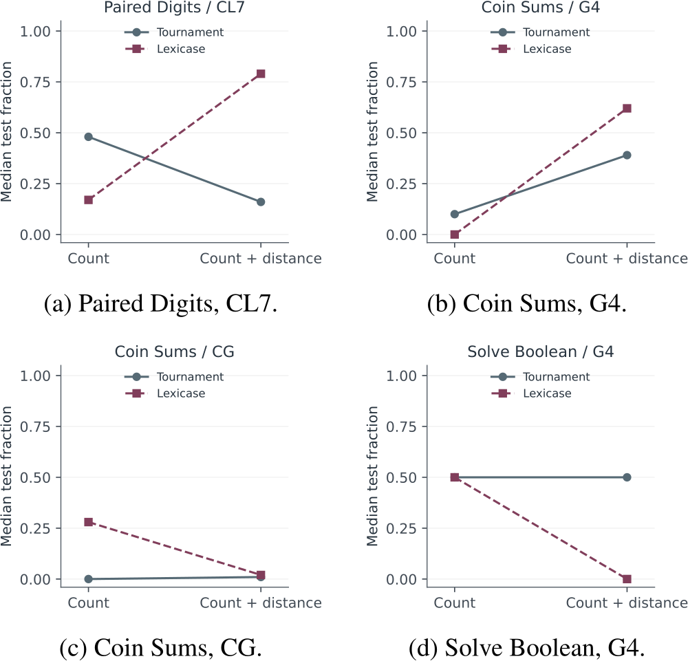
The Paired Digits row for CodeLLaMA is the largest example. TF, LF, TE, and LE have printed fractions 0.48, 0.17, 0.16, and 0.79. Changing selection alone produces a difference of -0.31, and changing fitness alone produces -0.32. Combining the changes produces a difference of 0.31 relative to TF. The interaction contrast is consequently 0.94. This value records the reversal between conditional effects, not a 94-percentage-point improvement over the initial generated program. The distinction matters because a large interaction may arise partly from poor performance of the two intermediate configurations.
An opposing arrangement occurs for Solve Boolean with GPT-4. Three configurations have a printed median of 0.50, while LE has 0.00. Neither single change improves the fraction, and the combined setting loses 0.50. Coin Sums demonstrates that task identity alone is also insufficient: its interaction is -0.27 for ChatGPT and 0.33 for GPT-4. For ChatGPT, LF reaches 0.28 but LE reaches only 0.02; for GPT-4, LF reaches 0.00 and LE reaches 0.62. The same configuration change therefore has opposite descriptive consequences under the two generator labels.
The contrasting slopes in Figure 1 express these conditional effects directly. Parallel slopes would indicate a zero interaction, while slope separation indicates a dependence of the fitness difference on selection. Their crossing for Paired Digits makes the inadequacy of adding the two single-change effects visible. The Coin Sums panels show why a general claim about one task’s response would overlook model-specific differences. The plots trace values between two discrete fitness settings solely to compare differences; they do not describe continuous trajectories through an evolving population.
Across the 43 pairs, seven interaction contrasts are positive, three are negative, and 33 equal zero at the displayed precision. The signed total is 0.83 and the mean is 0.01930. Removing the Paired Digits pair subtracts 0.94 from that total, changing the remaining mean to -0.00262. Thus the positive mean interaction is not evidence of consistently beneficial cooperation between fitness and selection. It is a balance of opposing effects in which one task contributes more than the entire positive net total.
B. Which Signs Survive Display Precision?
Six positive and three negative interactions remain strictly separated from zero under the half-width 0.005 convention. The positive Bowling–ChatGPT contrast of 0.02 has enclosure [0.00, 0.04], so its sign is unresolved. The other large contrasts are well separated: Paired Digits–CodeLLaMA lies in [0.92, 0.96], Solve Boolean–GPT-4 in [-0.515, -0.480], and Coin Sums–ChatGPT in [-0.285, -0.250]. Their directions cannot be reversed by any values inside the specified display intervals.
| Task | Model | \(D\) | Lower | Upper |
|---|---|---|---|---|
| Bouncing Balls | L3 | -0.020 | -0.030 | -0.010 |
| Bowling | L3 | 0.100 | 0.080 | 0.120 |
| Bowling | CG | 0.020 | 0.000 | 0.040 |
| Coin Sums | CG | -0.270 | -0.285 | -0.250 |
| Coin Sums | G4 | 0.330 | 0.310 | 0.345 |
| Cut Vector | CL7 | 0.070 | 0.055 | 0.085 |
| Leaders | CL7 | 0.120 | 0.100 | 0.140 |
| Paired Digits | CL7 | 0.940 | 0.920 | 0.960 |
| Snow Day | G4 | 0.040 | 0.020 | 0.060 |
| Solve Boolean | G4 | -0.500 | -0.515 | -0.480 |
The intervals in Table 2 are not uniformly symmetric because clipping affects rounded endpoints while integer endpoints remain fixed. For Coin Sums with ChatGPT, the TF token 0.00 permits a small positive value but no negative fraction. For GPT-4 on the same task, the LF token is also 0.00. This token-level information changes the interval endpoints even though ordinary floating-point conversion would make integer zero and rounded zero numerically indistinguishable. Preserving the printed representation is therefore a substantive part of the precision analysis.
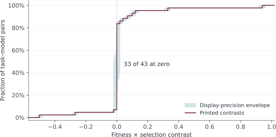
The cumulative distribution in Figure 2 separates the concentration at zero from the widely spaced nonzero values. The zero group is much larger than the combined positive and negative groups, but this does not establish exact equality of the unrounded medians. Some zero contrasts combine identical integer endpoints, while others combine rounded values that could conceal a small positive or negative difference. The envelope bounds the cumulative fraction using the interval endpoints. It expresses display uncertainty and supplies no sampling-based probability for the observed interaction signs.
C. Average Ranking and Weighting Sensitivity
LE has the highest average under each weighting scheme. Equal-task weighting gives means of 0.26375, 0.25528, 0.25000, and 0.29157 in configuration order. Equal-model weighting gives 0.25323, 0.25779, 0.25879, and 0.27198. The ordering of the other three configurations changes, showing that their relative means depend on composition. Equal-task weighting increases the contribution of tasks represented by only one eligible model, including Paired Digits, whereas equal-pair weighting gives more total influence to tasks represented by all four models.
c
| Weighting | TF | LF | TE | LE |
|---|---|---|---|---|
| Equal pair | 0.24163 | 0.24395 | 0.24372 | 0.26535 |
| Equal task | 0.26375 | 0.25528 | 0.25000 | 0.29157 |
| Equal model | 0.25323 | 0.25779 | 0.25879 | 0.27198 |
The changes among TF, LF, and TE illustrate how a small difference can be an artifact of aggregation even when every input value is correctly transcribed. Equal-task weighting ranks TF ahead of both alternatives, while equal-model weighting places TE ahead of LF and TF. There is no contradiction between these calculations: each averages the same cell values with a different distribution of importance. Their disagreement is a reason to state the weighting rule rather than report an unexplained grand mean. LE remains first under the three rules, which supports a more limited and transparent ranking claim.
The agreement concerning LE in Table 3 survives the display intervals. Its lower mean enclosure exceeds every competitor’s upper mean enclosure under all three weightings. Under equal-pair weighting, for example, the LE lower endpoint is 0.26198, while the largest competitor upper endpoint is 0.24756. This is a deterministic separation under the stated precision convention. It neither estimates the uncertainty of the underlying ten-run medians nor resolves how a different collection of tasks would change the ranking.
D. Worst Losses and Randomized Choice
The rowwise best mean is 0.28372. Comparing each fixed action with the best action in every row gives average regrets of 0.04209 for TF, 0.03977 for LF, 0.04000 for TE, and 0.01837 for LE. Their maximum regrets are 0.52, 0.62, 0.63, and 0.50. LE is therefore the best fixed choice under both criteria. Nevertheless, the difference between its average and maximum loss remains consequential: a small mean regret coexists with a loss equal to half of the test-fraction range on the least favorable observed pair.
The nominal minimax distribution assigns probabilities 0.27278 to TF, 0.10467 to LF, 0.14321 to TE, and 0.47935 to LE. Its maximum regret is 0.23967, compared with 0.50 for fixed LE. The reduction is 0.26033, or approximately 52.1% of LE’s maximum regret. Its mean utility is 0.25354 and its average regret is 0.03018. Randomization consequently exchanges 0.01181 of average median-score utility for a lower observed maximum loss. The calculation does not establish that this exchange is preferable for every software-development objective.
| Choice | Mean utility | Mean regret | Maximum regret |
|---|---|---|---|
| TF | 0.24163 | 0.04209 | 0.52000 |
| LF | 0.24395 | 0.03977 | 0.62000 |
| TE | 0.24372 | 0.04000 | 0.63000 |
| LE | 0.26535 | 0.01837 | 0.50000 |
| Uniform distribution | 0.24866 | 0.03506 | 0.39000 |
| Nominal minimax | 0.25354 | 0.03018 | 0.23967 |
| Precision-aware minimax | 0.25353 | 0.03019 | 0.24120 |
The losses in Table 4 are evaluated at the printed medians, including the precision-aware distribution. Its nominal maximum of 0.24120 should not be confused with the maximum over its interval box, 0.24586. The uniform distribution improves maximum regret relative to every fixed action but remains inferior to the optimized distribution under both mean and maximum regret. Unequal probabilities matter because the adverse rows have unequal outcome differences. Treating all configurations symmetrically would ignore these differences rather than provide additional protection.
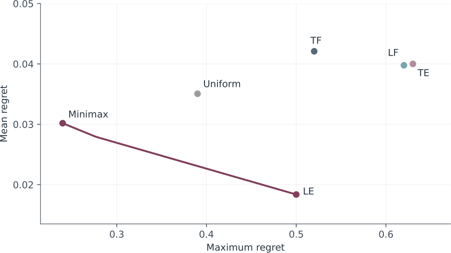
The feasible trade-off in Figure 3 shows how average regret changes when its maximum is capped. At one end, the nominal minimax distribution attains the smallest feasible maximum. Relaxing that restriction permits distributions with lower average regret, ultimately reaching fixed LE. The intervening line is calculated by solving constrained linear programs, not by interpolating an empirical learning curve. Its interpretation is restricted to the four available actions and the recorded utility matrix, but it makes the decision consequence of a loss cap explicit.
E. Adverse Rows that Determine the Probabilities
Four pairs attain the nominal minimax maximum simultaneously: Coin Sums with ChatGPT, Coin Sums with GPT-4, Paired Digits with CodeLLaMA, and Solve Boolean with GPT-4. Their equal losses of 0.23967 identify the competing demands determining the distribution. Greater LE probability protects Paired Digits and GPT-4 Coin Sums but worsens GPT-4 Solve Boolean. Greater LF probability protects ChatGPT Coin Sums but is costly on the GPT-4 version of that task. TF and TE enter the compromise because their losses across these competing rows differ.
The active rows also distinguish local evidence from a model-wide recommendation. GPT-4 appears twice with opposed demands: its Coin Sums row favors LE, whereas its Solve Boolean row penalizes LE. A policy selected solely from the generator name cannot resolve this conflict without additional information about the task or the program. The ChatGPT Coin Sums row further shows that sharing a task name does not imply sharing the same favorable configuration. These observations locate the decision difficulty in the joint task–model outcomes, while leaving the interpretation of generator differences descriptive rather than causal.
The presence of all four actions in the optimal distribution does not mean they are equally effective or that all are needed for every repair. TE, for example, has the largest maximum regret as a fixed action but remains useful in combination because it performs better than LF on GPT-4 Coin Sums while preserving the Solve Boolean fraction. This is a decision-level complementarity among action utilities. It does not establish complementarity among individual patches, because no joint distribution of patches or successful test cases is available.
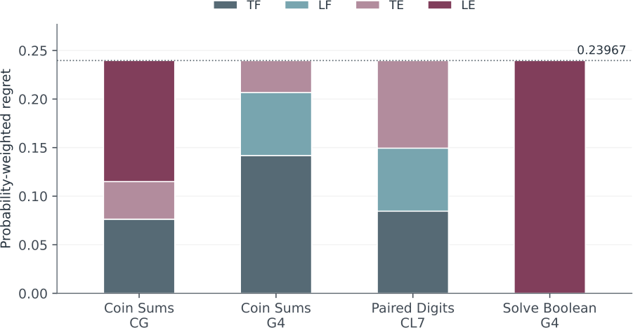
The constraint contributions in Figure 4 make this balance visible without implying an execution sequence. Each stack partitions the randomized rule’s regret into probability-weighted differences from that row’s best printed configuration. The equal totals are an optimization property. The distinct internal compositions explain why simply shifting more probability toward the action with the highest mean cannot continue indefinitely while preserving the minimax bound. The design thereby connects the mathematical constraints to the specific tasks determining the result.
F. Precision-Aware Choice and Task Deletion
Allowing the medians to vary within their display intervals changes the probabilities to 0.27083, 0.10965, 0.14081, and 0.47871 in configuration order. The corresponding worst interval regret is 0.24586. By comparison, applying the nominal probability vector to the interval box gives 0.24726. The adjustment therefore improves the interval guarantee by approximately 0.00140, with negligible change in average utility. Doubling the half-width to 0.01 increases the optimized bound to 0.25200. This wider enclosure preserves the qualitative trade-off while confirming that the exact probabilities and guaranteed loss depend on the specified display tolerance.
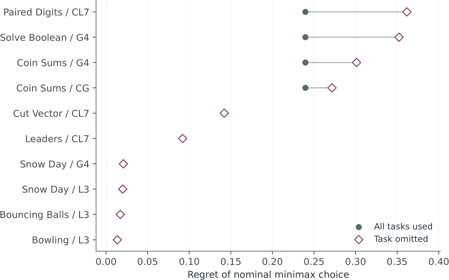
Task deletion gives a more substantial change. The nominal minimax rule has mean regret 0.03781 and maximum regret 0.36167 across the omitted rows. The precision-aware rule gives 0.03786 and 0.36294 when evaluated at the printed medians. The mean-maximizing rule chooses LE in every task deletion and retains mean regret 0.01837 and maximum regret 0.50. These results preserve the direction of the observed trade-off but weaken the apparent protection achieved when every adverse task is available during fitting.
| Fitted rule | Mean utility | Mean regret | Maximum regret |
|---|---|---|---|
| Maximum mean | 0.26535 | 0.01837 | 0.50000 |
| Nominal minimax | 0.24591 | 0.03781 | 0.36167 |
| Precision-aware minimax | 0.24586 | 0.03786 | 0.36294 |
The omitted-task losses in Table 5 are most unfavorable for Paired Digits, Solve Boolean, and Coin Sums. Removing Paired Digits produces regret 0.36167 on its CodeLLaMA row; removing Solve Boolean produces regret 0.35227 on its GPT-4 row. These cases show that an adversarial rule can depend strongly on having encountered the adverse condition it protects against. The difference is a limitation of the observed support, not a numerical failure of the optimization.
The task-deletion comparison in Figure 5 separates losses obtained when all tasks contribute to fitting from losses obtained after a whole task is withheld. The largest changes occur among rows that determine the full-data optimum. Removing many other tasks leaves the nominal minimax probabilities unchanged. The graphic thus distinguishes ordinary low-influence rows from the small set carrying the worst-loss compromise. It should not be read as a confidence interval or as a forecast of deployment performance.
IV. Discussion
A. Why a Combined Configuration does not Identify a Mechanism?
The four-cell evidence provides a stronger descriptive statement than a comparison between TF and LE alone. It identifies whether the fitness difference changes with the selection procedure and reveals cases where both single changes are unfavorable but their combination is favorable. However, attributing such a pattern to a specific search mechanism would require information about populations, selected parents, candidate programs, and casewise errors. The medians contain none of these trajectories. A positive interaction therefore establishes a nonadditive outcome pattern, while the explanation in terms of preserved specialists or useful discrepancy gradients remains a hypothesis.
Paired Digits illustrates this boundary well. Its interaction of 0.94 is large because LE improves over TF and because both intermediate configurations perform much worse. Describing only the final improvement would miss the two unfavorable intermediate outcomes. Describing the interaction as a causal amplification would go beyond the available evidence. A responsible interpretation is that the effect of replacing count fitness is strongly conditional on selection in this task–model pair. The record supports a configuration-specific comparison, not a universal recommendation to add either component independently.
The negative Coin Sums and Solve Boolean cases also matter for methodological interpretation. A more detailed output discrepancy need not align with program modifications that solve the task under every selection procedure. Likewise, retaining candidates that perform well on particular cases does not guarantee that subsequent variation assembles a broadly correct program. The present calculations cannot determine which of these mechanisms operated, but they show why the mechanism cannot be inferred from the name or apparent sophistication of the configuration. Opposing interactions should remain part of the interpretation even when the average favors LE.
B. Selecting a Loss Criterion before Choosing a Configuration
The fixed-choice result is precise: LE maximizes the mean under all three weightings and minimizes maximum regret among deterministic choices. The randomized result answers a different preference. It permits a lower average score to reduce exposure to the most unfavorable row. Neither result supplies a universal ranking independent of the decision objective, consistent with the distinction between selection and portfolio construction [22]. A user who values average test fraction across the eligible collection would choose LE; a user who accepts median-score utilities and prioritizes the specified maximum regret would choose the optimized distribution.
A further distinction concerns regret and absolute quality. A task on which every configuration scores zero has zero regret under every distribution, despite its complete lack of test success. Conversely, a relatively high score can incur substantial regret when another configuration performs much better. Regret measures avoidable loss within the available action set. It does not measure unresolved software risk, semantic correctness, or fitness for release. Any operational use would therefore need an independent adequacy criterion in addition to the configuration-choice rule. The present paper supplies no threshold for accepting a repaired program.
This distinction is consistent with evidence on test-suite overfitting in program repair. Generating additional tests can reveal patches that satisfy the repair tests while remaining incorrect [36]. Detailed examination of test-based patch acceptance likewise questions when passing tests warrants accepting a change [37]. These findings concern the validity of the program-level outcome, whereas minimax regret concerns which configuration to choose among the observed outcomes. Combining the two questions would obscure their separate information requirements. No regret guarantee can compensate for a test collection that fails to express important required behavior.
C. What the Precision Bounds Establish?
The interval calculations establish that the principal opposing signs and the best average configuration are insensitive to the stated display precision. They do not establish low experimental uncertainty. Ten runs can yield a median with considerable variability across repeated execution campaigns, even when that median is printed to several decimal places. Conversely, coarse printing can obscure a stable small difference. Numerical precision and sampling variability are different properties, and the present intervals address only the former. Their narrow widths cannot justify claims of statistically precise repair performance.
The shared-coordinate cancellation in the regret calculation has a practical consequence. The same unknown median must be used when an action appears both as a rival and as part of the randomized choice. If the action is selected with probability one, its regret against itself is exactly zero. Allowing two independent values for that single median would create a spurious positive self-loss. Retaining the common coordinate produces the stated linear constraints and permits exact verification by enumerating the interval-box corners. This detail is essential for a numerically correct bound, especially near deterministic distributions.
The task-deletion findings address a different uncertainty: dependence on which tasks are present. The distribution changes sharply when an adverse task is removed, even though the display intervals produce only small adjustments. That contrast shows that observing the right types of configuration failure matters more here than refining the last printed decimal. It also explains why the full-collection bound cannot be transferred to new software. The adverse set outside the 18 represented tasks is unspecified, so its maximum regret is not constrained by the reported optimum.
D. Evaluation Boundaries and Research Implications
Task composition is central because repair eligibility depends on initial failure. Dehghani et al. show how evaluation choices can alter apparent algorithm superiority [38]. In this record, stronger initial screening performance leaves a smaller conditional repair collection. Equal-model weighting prevents one label from receiving more total weight simply because it has more eligible pairs, but it cannot recreate the missing outcomes for initially solved combinations. The analysis consequently addresses configuration choice among difficult eligible cases, not the end-to-end value of selecting a language model and then applying repair.
Holding out complete tasks avoids one obvious way of sharing related outcome information between fitting and evaluation. It does not remove every form of selection dependence, because the research question and analytical choices were developed after inspecting the same published collection. Work on leakage in machine-learning-based science emphasizes the importance of respecting information boundaries throughout study design [39]. Cross-validation research also shows that the quantity estimated depends on the fitting and evaluation procedure [40]. These considerations support describing the deletion results as sensitivity evidence and reserving external-performance claims for a separate task set.
The analysis identifies specific priorities for an independent evaluation. Run-level records should preserve selected programs, random seeds, task identifiers, and per-configuration evaluation costs. A randomized configuration policy should be fixed before generating those outcomes, and its utility should be defined in terms of the observed run-level quantity of interest. Such an evaluation could determine whether reducing maximum median-score regret also reduces unfavorable execution outcomes. These requirements follow from the present limitations; they are not additional experiments claimed in this manuscript.
An additional interpretive constraint follows from using medians. Averaging the four action medians with selection probabilities is mathematically well defined even when the underlying distributions are unavailable. However, its legitimacy as a decision utility is a preference assumption, not a recovered property of those distributions. The calculated probabilities require an explicit utility definition wherever they appear. Reporting them alone could suggest a stronger empirical result than was obtained, particularly if a reader assumes that the same numbers optimize expected individual-run correctness or guarantee a particular probability of successful repair. Such interpretations require separate evidence.
The finite support imposes another practical boundary. A task with no observed configuration differences contributes nothing to the choice distribution, even if it is intrinsically difficult or computationally expensive. This behavior follows from the regret objective and should not be mistaken for a judgment that the task is unimportant. Adding an absolute-quality requirement, a runtime penalty, or a minimum probability of complete correctness would alter the optimization problem. Those additions could be sensible with appropriate evidence, but they are not silently encoded in the reported probabilities. The current result is tied to one explicit utility definition [23].
The main contribution is consequently narrow but reproducible. The published four-configuration arrangement contains opposing interactions that a two-configuration comparison cannot describe. Those interactions create a measurable conflict between average utility and maximum avoidable loss. The included arithmetic, linear programs, and task-deletion records make that conflict inspectable without reconstructing unavailable run histories. The decision analysis remains useful precisely because its unit, utility definition, and uncertainty set are stated explicitly rather than treated as interchangeable descriptions of repair success.
V. Conclusion
The research question concerned configuration choice when fitness and selection interact and only rounded median test fractions are available. The finite collection supports two answers tied to explicit objectives. LE is the preferred fixed configuration: it has the highest mean under equal-pair, equal-task, and equal-model weighting and the smallest maximum regret among fixed actions. Its favorable mean nevertheless coexists with a maximum regret of 0.50, driven by a substantial failure on Solve Boolean with GPT-4.
A randomized choice over configuration-level median utilities reduces the observed maximum regret to 0.23967 while decreasing mean utility from 0.26535 to 0.25354. Display-precision uncertainty changes the optimized bound to 0.24586, whereas withholding complete tasks raises the nominal rule’s maximum regret to 0.36167. The dominant limitation is therefore dependence on the observed adverse tasks rather than the final decimal place of their printed scores. Opposing interactions, especially Paired Digits and Solve Boolean, explain why a favorable combined average cannot be interpreted as universal cooperation between fitness and selection.
The resulting conclusion is a bounded decision claim: fixed LE suits the stated average-score objective, while a minimax distribution suits a preference for limiting the largest observed avoidable loss under the defined utility model. Neither choice guarantees program correctness, and the randomized result is not an execution-level performance claim. Independent run-level evaluation is needed before translating this calculated trade-off into a recommendation for a deployed repair system.
Data and Code Availability
The accompanying project contains the 172 token-preserving configuration records, all calculated contrasts and decision outputs, plotting code, and compilation files.
Conflict of Interest
The author declares no conflict of interest.
Declaration of Generative AI Use
During the preparation of this study, the author used Claude (Anthropic), an artificial intelligence based language model, to assist with the development and refinement of R code. All AI generated outputs were critically reviewed, edited, and, where necessary, rewritten by the author. The author independently verified all statistical analyses and figures against the underlying R output and takes full responsibility for the content, accuracy, interpretation, and conclusions presented in this publication.