
Electricity is traded under a distinctive combination of limited short-run storability, network constraints, inelastic demand, weather-dependent supply, and market clearing at finely resolved delivery periods. These properties produce serial dependence, strong intraday and weekly seasonality, time-varying variance, negative prices, and occasional upward excursions that are large relative to the prevailing level. A single expected price cannot communicate the asymmetric exposure created by those features. Traders need a range for revenue and imbalance calculations, retailers need a range for procurement and tariff decisions, producers need it for commitment and maintenance planning, and system-facing analysts need it to distinguish an ordinary forecast error from a change in the operating state. Probabilistic forecasts therefore matter not because point accuracy is unimportant, but because price-sensitive decisions are made before the delivery-hour outcome is known.
The forecasting literature has progressed from autoregressive specifications and neural point predictors toward high-dimensional machine learning and explicit distributional forecasts. Reviews consistently report that careful temporal validation, market-specific preprocessing, and transparent comparison rules often matter as much as the chosen algorithm [1]–[3]. Early neural comparisons established the sensitivity of day-ahead accuracy to architecture and input selection [4]. Regularized autoregression can recover the structured dependence between the 24 hourly auctions of adjacent days [5], while integrated-market covariates and deep architectures can improve performance where neighboring zones transmit information [6], [7]. Neural autoregressive density models, recurrent spline quantiles, attention-based multi-horizon networks, diffusion models, and copula-based estimators broaden the distributions that can be represented [8]–[12]; the expanding transformer literature further emphasizes long-range representation and computational tradeoffs [13]. Their flexibility, however, does not itself guarantee that a nominal 90% interval will contain approximately 90% of subsequently observed prices.
Electricity-price uncertainty is particularly difficult to calibrate because the forecast-error distribution is not stable. A price model estimated in a high-load winter can be too diffuse in a mild summer and too narrow during a later supply shock. An interval fitted to the whole sample may report acceptable average coverage even when its errors cluster at specific hours or regimes. Such averaging is operationally consequential. System demand changes predictably over a day, yet the price response to a demand increment depends on the generation stack and available flexibility. The same absolute residual may be routine at the evening peak and exceptional overnight. A method that treats all calibration residuals as equally informative ignores that local structure.
Quantile regression offers a direct route to heterogeneous intervals. Instead of imposing constant Gaussian variance, it estimates conditional lower and upper quantiles by minimizing asymmetric pinball losses [14]. Tree boosting accommodates nonlinear interactions without requiring an a priori parametric price equation [15]. The resulting endpoints may still be miscalibrated because finite training data, distribution shift, hyperparameter selection, and approximation error displace estimated quantiles from their intended probabilities. Published price applications accordingly report persistent tension between coverage and width [16]–[18]. This tension should be assessed with a proper interval score in addition to coverage, because an arbitrarily wide interval can cover almost everything while conveying little usable information [19].
Conformal prediction separates predictive modeling from empirical calibration and has become an accessible model-agnostic approach to uncertainty quantification [20]. For exchangeable observations, a held-out set of conformity scores supplies a finite-sample correction that can wrap around almost any regression algorithm. Conformalized quantile regression preserves the local width produced by conditional quantiles and adds a scalar correction derived from calibration errors [21]. Related theory clarifies when locally adaptive intervals remain efficient [22], [23]; recent work also distinguishes aleatoric variability from uncertainty in estimated conditional quantiles [24]. General regression results establish distribution-free predictive inference under limited assumptions [25]. Electricity observations ordered in time are neither independent nor generally exchangeable, so a static correction can become stale. Research on covariate shift [26], non-exchangeable sequences [27], and online distribution shift [28], [29] shows how calibration can be modified when recent errors carry different information from distant ones.
Several time-series conformal procedures update intervals as outcomes arrive. Ensemble batch prediction intervals use leave-one-out residuals and online updating for dependent sequences [30]. Conformal time-series forecasting explicitly addresses temporal structure [31]. Adaptive conformal inference changes its effective miscoverage level following recent successes and failures, while expert aggregation reduces dependence on a single learning rate [32]. Strongly adaptive online learning further targets performance over multiple time scales [33], and multi-step adaptations distinguish errors at different horizons [34]. These contributions establish that a chronological calibration mechanism is preferable to random resampling when the intended use is forward forecasting. They also leave a practical design choice: should the correction respond only to when an error occurred, or also to whether that error arose under conditions resembling the forthcoming delivery hour?
The attached electricity-price study illustrates the value of reporting intervals and state probabilities rather than only point forecasts, but it relies on discrete dynamic Bayesian states and a short Danish evaluation window [35]. The present paper pursues a different question, geographical market, observation span, estimator, and validation design. It examines whether a continuous quantile model can be calibrated by selecting the historical errors that are most relevant to the current operating condition. The empirical record covers four years of French hourly prices rather than a one-day holdout, and the assessment advances one hour at a time through a complete unseen calendar year. This longer horizon exposes seasonal changes, daylight-saving transitions, calm periods, and price excursions that a brief test cannot reveal.
The central research question is: Can a conformal correction weighted jointly by recency and operating similarity achieve near-nominal annual coverage with materially narrower intervals than a single global split-conformal correction? The question has three subsidiary aspects. First, the correction should improve on the severe undercoverage of raw conditional quantiles. Second, any gain in sharpness relative to global calibration should not be purchased through broad systematic undercoverage across delivery hours or months. Third, adaptation should be interpretable: the correction should expand when recent, hour-matched, demand-matched, and volatility-matched errors justify expansion, rather than through an opaque auxiliary neural layer.
To answer the question, this study introduces recency- and operating-condition-weighted conformal calibration (ROWCC). Three histogram gradient-boosting models estimate the 0.05, 0.50, and 0.95 conditional price quantiles. The base interval is enlarged by a weighted 0.90 quantile of preceding nonconformity scores. Each score receives a time-decay weight, a delivery-hour weight, and smooth similarity weights for system consumption and the standard deviation of the preceding 24 hourly prices. A small global anchor prevents local estimates from becoming erratic when effective weight is low. Once an observed price becomes available, its score enters the history and can affect later intervals; no future outcome is used.
The contribution is empirical and methodological. Methodologically, the procedure joins heterogeneous quantile estimation with a calibration rule that has a direct operational interpretation. It differs from a global conformal adjustment because relevant residuals need not contribute equally, and it differs from pure adaptive-miscoverage recursion because current covariates influence the calibration weights before the price is observed. Empirically, the study provides a full-year chronological test with annual, monthly, hourly, and high-price diagnostics. The conclusion is deliberately conditional rather than universal: ROWCC substantially improves the reliability–sharpness balance for the observed French market record, while the rare upper tail remains harder to cover than the annual average suggests.
The remainder of the paper is organized as follows. Section II defines the market record, temporal partitions, predictors, and evaluation measures. Section III presents quantile boosting, static conformal calibration, and ROWCC in mathematical form. Section IV reports aggregate and conditional results, interprets each figure and table, and discusses practical implications. The conclusion returns directly to the research question.
The record contains 34,896 consecutive hourly observations from 8 January 2016 at 00:00 through 31 December 2019 at 23:00. Prices are French day-ahead spot prices in EUR/MWh. The accompanying predictors comprise the delivery hour, seven day-of-week indicators, system consumption, the complete vector of 24 prices observed one day earlier, and the complete vector of 24 prices observed one week earlier[32]. The first seven days of 2016 are absent because the weekly lag vector must be fully observed before the first eligible forecast row. No interpolation is required in the supplied matrix. Across the full record, the mean price is 42.90 EUR/MWh and the standard deviation is 20.33 EUR/MWh; the observed range extends from \(-31.82\) to 874.01 EUR/MWh.
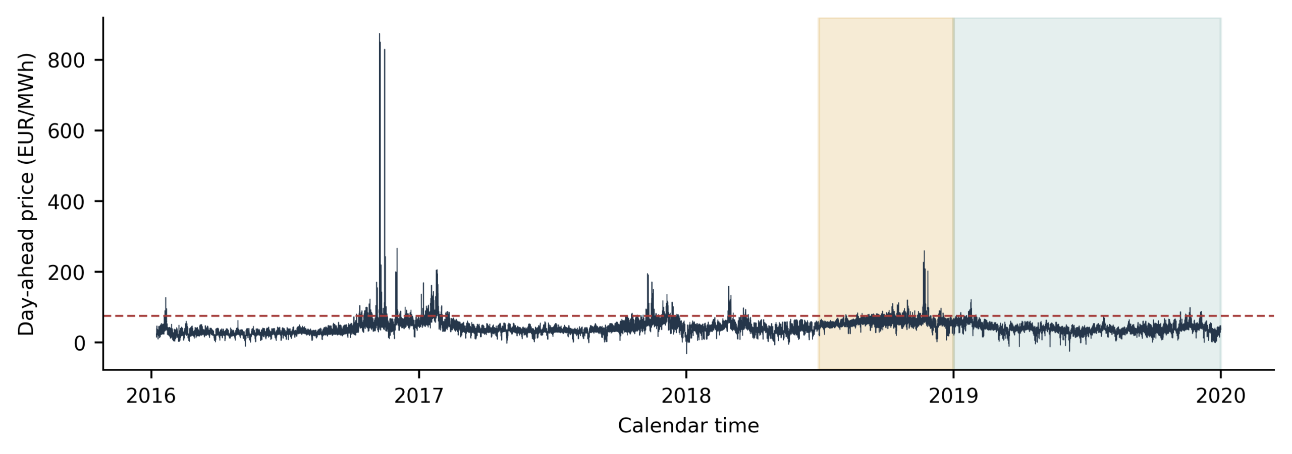
The chronological split is fixed before any model comparison. Observations through 30 June 2018 estimate the three conditional quantile functions. This estimation set contains 21,720 hours. The 4,416 hours from 1 July through 31 December 2018 form the initial conformal calibration set. The 8,760 hours of 2019 constitute the test set. At test time, forecasts are evaluated in timestamp order. An observed test score becomes eligible only after its price has been revealed. This protocol replicates the information sequence of deployment: model coefficients remain fixed during 2019, whereas the calibration distribution can learn from newly realized errors.
The separation between estimation and calibration is essential. Reusing training residuals would make the conformity scores optimistic because gradient boosting is optimized on those observations. A random calibration split would mix later and earlier regimes and would allow a past delivery forecast to be calibrated by residuals from its future. The chosen six-month calibration window supplies all delivery hours and weekdays across two seasons while remaining adjacent to the test year. The full test year avoids selecting an unusually favorable short episode.
The price chronology in Figure 1 shows why year-round evaluation is demanding. Most observations occupy a relatively compact band, but isolated excursions are far above the typical level and several negative prices occur. The shaded middle period denotes initial calibration, whereas the final shaded period denotes the untouched 2019 test. The horizontal threshold at 75 EUR/MWh is the 95th percentile of estimation prices and is fixed without inspecting test outcomes. This threshold later defines a diagnostic high-price subset. Its purpose is not to tune the method but to reveal whether annual coverage hides one-sided failures during commercially important events.
The partition statistics in Table 1 confirm that almost two thirds of the eligible observations estimate the predictive quantiles, roughly one half-year establishes the initial score distribution, and exactly one calendar year evaluates performance. The large maximum relative to the mean cautions against interpreting range-normalized width alone. For that reason, the analysis reports width in EUR/MWh, a normalized width for continuity with interval-forecasting practice, and a proper interval score.
| Segment | Period | Hours | Role |
|---|---|---|---|
| Estimation | 8 Jan 2016–30 Jun 2018 | 21,720 | Quantile-model fitting |
| Calibration | 1 Jul 2018–31 Dec 2018 | 4,416 | Initial conformity scores |
| Test | 1 Jan 2019–31 Dec 2019 | 8,760 | Chronological evaluation |
The predictor vector is available before the forecasted price is evaluated. It contains the scalar hour index; seven day-of-week indicators; the 24 prices from the corresponding day-ahead vector one day earlier; the 24 prices from one week earlier; and system consumption. Six derived covariates summarize structure that a finite tree ensemble would otherwise need to reconstruct repeatedly: mean, standard deviation, and range of the preceding-day vector; mean and standard deviation of the preceding-week vector; and an interaction between consumption and an indicator for delivery hours 07:00–20:00. These derived variables do not introduce outside information. They compress the amplitude and dispersion of already available lags and allow shallow tree partitions to recognize calm and volatile operating conditions.
The design deliberately avoids contemporaneous realized generation, fuel prices released after gate closure, or future price aggregates. Such variables could improve an ex post fit while weakening the forecast interpretation. System consumption is retained as supplied in the public forecasting matrix. Consumption and preceding-day volatility are also used by the calibration rule, but in a different role: the predictive model maps them to conditional price quantiles, whereas the calibration rule uses them to judge which historical errors are comparable to the current forecast.
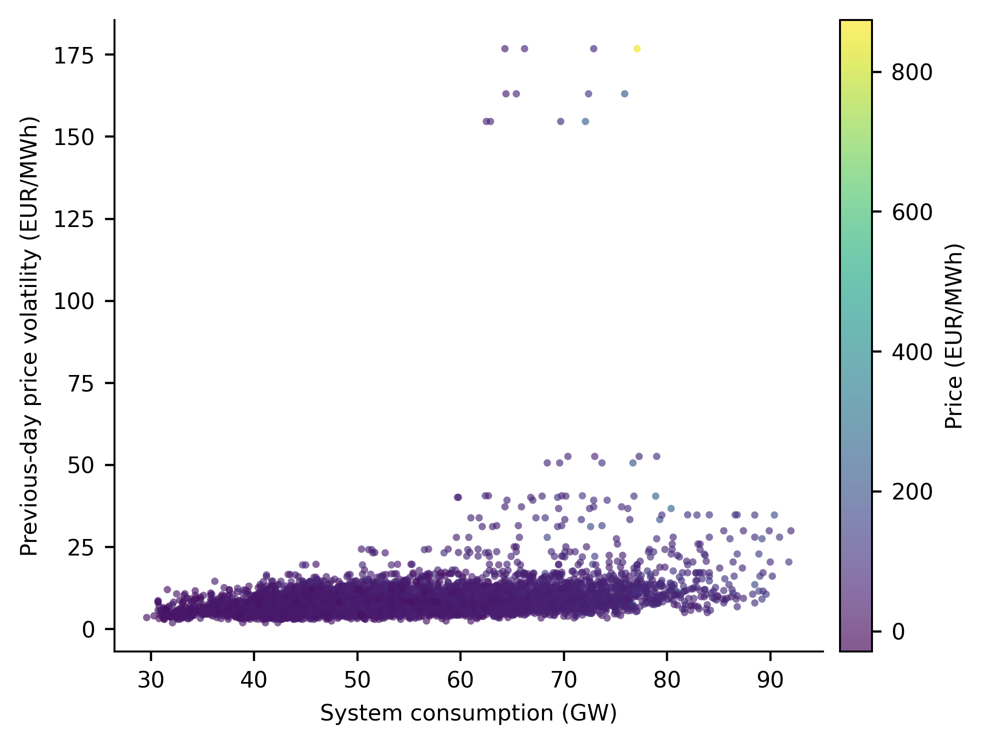
The operating plane in Figure 2 plots a systematic one-in-six subsample to preserve visual legibility. Higher prices appear across several demand levels, but dense high-consumption and high-volatility regions contain visibly more elevated outcomes. The pattern does not support a simple monotone demand-price equation. It instead supports a local calibration rule in which both demand proximity and volatility proximity affect relevance. A residual observed at moderate consumption after a calm preceding day should contribute less to the correction of a high-consumption forecast following a volatile day than an otherwise recent and hour-matched residual.
Let \(y_t\) denote the realized price and \([L_t,U_t]\) a nominal \((1-\alpha)\) interval, with \(\alpha=0.10\). Empirical coverage is
The mean interval width is \(\mathrm{MIW}=n^{-1}\sum_t(U_t-L_t)\). The normalized width divides MIW by the observed test range. Because a single extreme observation can enlarge that denominator, PINAW is treated as a supplementary descriptive statistic rather than the principal sharpness criterion.
Coverage and width are combined through the central interval score
The score rewards narrow intervals but penalizes misses in proportion to their distance beyond an endpoint. Lower values are better. Unlike an arbitrary weighted sum of coverage and width, it is a proper scoring rule for central prediction intervals [19]. Under- and over-rate are reported separately to expose directional error. Median point forecasts are evaluated by mean absolute error and root mean squared error, although the research question concerns interval calibration.
Aggregate annual statistics can conceal temporal concentration. Monthly coverage and width test seasonal stability; hour-specific statistics test whether morning and evening ramps receive adequate uncertainty; and the high-price subset tests the upper tail. The latter contains test outcomes at or above 75 EUR/MWh, a cutoff established exclusively from the estimation sample. Because this conditional subset is intentionally rare, its coverage is diagnostic and is not expected to inherit a marginal conformal guarantee.
For a quantile level \(\tau\in(0,1)\), the conditional quantile function \(q_{\tau}(x)\) minimizes the expected pinball loss
Separate histogram gradient-boosting regressors estimate \(\tau=0.05\), \(0.50\), and \(0.95\). The lower and upper models form the raw 90% interval, and the median model supplies the point forecast. Histogram binning accelerates repeated tree splits and reduces sensitivity to minute numeric changes. Each model uses 220 boosting iterations, learning rate 0.055, at most 31 terminal leaves per tree, a minimum of 35 observations per leaf, and \(L_2\) regularization 0.2. A fixed random seed controls implementation-level randomness. Hyperparameters are held constant across quantiles.
Tree ensembles are suitable here because lagged prices, delivery hour, and consumption can interact through thresholds. A morning price may respond differently to the same consumption level depending on whether the preceding-day vector contains a spike. The models do not assume linearity or constant error variance. They also avoid separate fits for each delivery hour, allowing information sharing across hours through the hour variable and its interactions. If independently fitted lower and upper quantiles cross, their endpoints are sorted before calibration. Crossings are rare in the test record but enforcing order makes every interval well-defined.
The estimator is intentionally less elaborate than many recent probabilistic neural systems. DeepAR represents autoregressive predictive distributions [8]; temporal fusion transformers combine gating, attention, and interpretable variable selection [10]; NBEATSx adds exogenous signals to basis expansions for price forecasting [36]; TimeGrad learns a diffusion process over future paths [11]; and TACTiS uses attentional copulas for multivariate dependence [12]. Those models are valuable when the goal is a rich joint distribution. The present goal is to isolate the effect of a transparent calibration rule on central hourly intervals, so an expressive but computationally moderate base learner is preferable.
Let \(\widehat q_{.05}(x_i)\) and \(\widehat q_{.95}(x_i)\) be fitted endpoints for a calibration observation. Its two-sided nonconformity score is
The score is positive when the observed price lies beyond the raw interval and negative when it lies inside both endpoints by a margin. With \(m\) calibration scores, the split-conformal correction is the upper empirical quantile at level
capped at one. The globally calibrated interval is
In the present calibration period, the correction is 6.50 EUR/MWh. It is applied symmetrically because the score already selects the larger endpoint violation. Under exchangeability, the finite-sample rank argument underlying conformalized quantile regression controls marginal miscoverage [21]. The time ordering here violates strict exchangeability, so global calibration is used as a conservative empirical comparator rather than as an unconditional theorem for 2019.
The attraction of the global correction is simplicity. Every calibration residual contributes equally, the correction is fixed, and the base quantile widths remain heterogeneous. Its limitation is equally clear: an error from July at 03:00 has the same influence on a December 18:00 forecast as a recent error under nearly identical consumption and volatility. If the calibration period is more difficult than the test period, the correction can remain unnecessarily large. If a new difficult regime emerges, it can remain too small until the model is refitted.
ROWCC replaces the unweighted empirical quantile by a forecast-specific weighted quantile. For forecast time \(t\) and a preceding scored observation \(i<t\), define age in days \(a_{it}\), delivery hours \(h_i\) and \(h_t\), consumption values \(d_i\) and \(d_t\), and preceding-day price standard deviations \(v_i\) and \(v_t\). The relevance weight is
with
Here \(\sigma_d\) and \(\sigma_v\) are standard deviations calculated only in the initial calibration period. The 42-day half-life allows an error to remain influential across several weekly cycles while gradually yielding to newer evidence. The nonzero hour weight and the 0.55 floors prevent the effective calibration set from collapsing when a condition is unusual. Exact hour matches nevertheless receive more than eight times the hour component of nonmatches.
The weighted empirical quantile \(Q^{(w_t)}_{1-\alpha}(s)\) is the smallest score whose cumulative ordered weight reaches \((1-\alpha)\) of total weight. To stabilize the correction, the forecast-specific value is anchored lightly to the original global correction:
The final interval is
For computational boundedness, at most the 5,000 most recent scored observations enter a forecast. Because the 42-day half-life makes older weights negligible, this truncation has little numerical effect while limiting sorting cost. All 4,416 initial calibration scores are present at the start of 2019. Each test score is appended only after its corresponding observed price is available.
This construction is related to adaptive conformal inference but does not update a single miscoverage parameter by a success/failure recursion. Instead, it changes the empirical score distribution presented to the quantile operation. The distinction matters when two forecasts occur close in time but under different delivery hours or volatility states. A pure time-recursive method would give them almost identical calibration states; ROWCC can give them different corrections. The construction is also related to covariate-weighted conformal ideas, but it uses smooth operational proximity and recency for sequential calibration rather than estimating a train-to-test density ratio.
The weighting parameters are fixed before test evaluation and are not optimized on 2019 coverage. This constraint prevents the annual test from becoming a tuning set. The chosen weights express three qualitative judgments: recent errors are more relevant, same-hour errors are substantially more relevant, and load or volatility dissimilarity should attenuate rather than eliminate an observation. A formal exchangeability guarantee does not follow from these heuristic weights. Accordingly, the paper evaluates coverage rigorously over time and states the inferential scope explicitly. Distribution-free terminology is reserved for the conformal rank mechanism under its assumptions, not for an unsupported claim that arbitrary market shifts are solved.
Three interval systems share the same lower and upper boosting models. Raw quantile boosting uses \([\widehat q_{.05},\widehat q_{.95}]\) without correction. Static CQR adds the constant 6.50 EUR/MWh calibration correction. ROWCC adds the forecast-specific correction \(q_t\). Since the predictive endpoints are identical before calibration, differences among systems isolate the calibration rule rather than changes in feature engineering, model capacity, or training period.
The analysis is implemented in Python with pandas, NumPy, scikit-learn, and Matplotlib. Dates are parsed once and never shuffled. Feature summaries are computed row-wise from lag variables already present. Quantile models see only the estimation segment. The static correction sees only the initial calibration segment. ROWCC begins with that same segment and updates sequentially. The test predictions, correction values, summary results, analysis script, and figure assets accompany the manuscript. This audit trail permits verification of every table entry without depending on a stochastic external service.
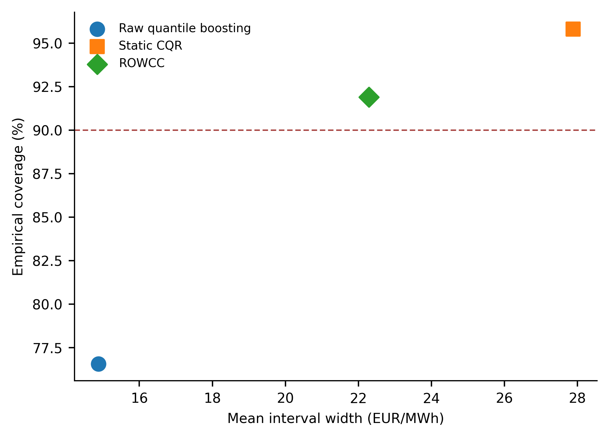
The aggregate results in Table 2 expose the calibration problem directly. Raw quantile boosting covers only 76.56% of 2019 prices, 13.44 percentage points below the nominal level. Its narrow 14.88 EUR/MWh mean width is therefore misleading if considered alone. Lower-tail and upper-tail misses are nearly balanced at 11.52% and 11.92%, indicating that the principal defect is not a single displaced endpoint; both tails are too close to the median for the subsequent year.
Global split calibration more than repairs the deficit. Coverage rises to 95.82%, with only 4.18% total miscoverage. The cost is a mean width of 27.88 EUR/MWh, an 87.41% increase over the raw interval. Because the global adjustment is symmetric, the width increases by twice the 6.50 EUR/MWh correction at every hour. Most remaining misses occur below the lower endpoint, whereas only 1.06% occur above the upper endpoint. This directional pattern suggests that the second half of 2018 contained calibration errors large enough to make the 2019 upper endpoint broadly conservative.
ROWCC occupies a preferable middle position. Its 91.91% annual coverage is 1.91 percentage points above nominal, while its 22.29 EUR/MWh mean width is 5.59 EUR/MWh narrower than global CQR, a reduction of 20.06%. Relative to raw quantile boosting, it recovers 15.35 percentage points of coverage for a 7.41 EUR/MWh increase in average width. The mean interval score is 28.94 EUR/MWh, lower than 32.41 for raw boosting and 31.52 for global CQR. The score comparison is important because it values both narrowness and the magnitude of misses: ROWCC does not merely move along an arbitrary coverage-width scale, but produces the best combined probabilistic performance under a proper scoring rule.
| Method | PICP (%) | MIW | PINAW (%) | IS | Below (%) | Above (%) |
|---|---|---|---|---|---|---|
| Raw quantile boosting | 76.56 | 14.88 | 10.16 | 32.41 | 11.52 | 11.92 |
| Static CQR | 95.82 | 27.88 | 19.05 | 31.52 | 3.12 | 1.06 |
| ROWCC | 91.91 | 22.29 | 15.22 | 28.94 | 5.09 | 3.00 |
MIW and IS are in EUR/MWh. All methods share the same median forecast, whose MAE is 4.84 EUR/MWh and RMSE is 6.45 EUR/MWh.
The coordinate view in Figure 3 makes the practical tradeoff visible without merging evaluation criteria into an opaque objective. Raw quantiles are sharp but unreliable. Static CQR is reliable but sits far to the right because of its uniform enlargement. ROWCC lies above the target-coverage line and substantially to the left of static CQR. The separation confirms that condition-sensitive calibration, rather than a different predictive model, causes the improvement.
All systems have the same median MAE of 4.84 EUR/MWh and RMSE of 6.45 EUR/MWh. This equality is a design feature rather than a limitation of the comparison. It prevents a more accurate point predictor from being mistaken for better calibration. The interval findings therefore answer a specific question: given fixed conditional quantiles and median, how should the residual uncertainty be corrected? ROWCC improves the answer without altering the underlying point path.
The normalized widths in Table 2 should be read cautiously. The 2019 observed range includes extremes, so the denominator is much larger than the central mass of prices. The absolute width and interval score are more stable for decision interpretation. A 5.59 EUR/MWh reduction from static CQR applies to every procured or generated megawatt-hour represented by the interval. Its commercial value depends on the decision rule, but its statistical meaning is unambiguous: less price space is declared plausible on average while the observed annual coverage remains above target.
The four-day window in Figure 4 is selected mechanically from the 2019 week with the greatest within-week price standard deviation; the displayed four days begin at that weekly boundary. The observed line moves rapidly and the median follows its main direction, although it smooths several local extrema. The interval does not maintain a constant distance from the median. Its base width changes with conditional quantile dispersion, and its conformal expansion changes with the weighted score history.
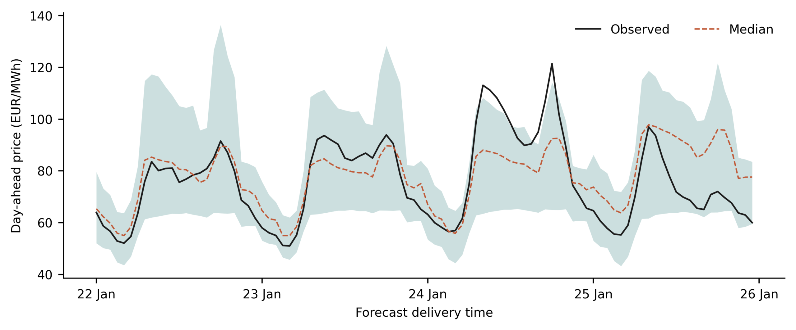
The episode demonstrates why two adaptation mechanisms are useful. Quantile boosting anticipates heteroscedasticity from lags and consumption, producing a wider raw band when the covariates indicate uncertainty. ROWCC then corrects any remaining local miscalibration using comparable preceding errors. A fixed Gaussian error variance could not create the same shape, while global CQR would simply add 6.50 EUR/MWh to both endpoints throughout the window. The adaptive band remains interpretable: its movement reflects model-implied conditional dispersion plus an empirically observed correction.
No individual episode establishes overall validity. The graphic is therefore paired with annual, monthly, and hourly summaries rather than presented as representative by assertion. The displayed outcome is useful because it shows actual interval behavior when prices change quickly, while the tables quantify how often that behavior succeeds across all 8,760 test hours.
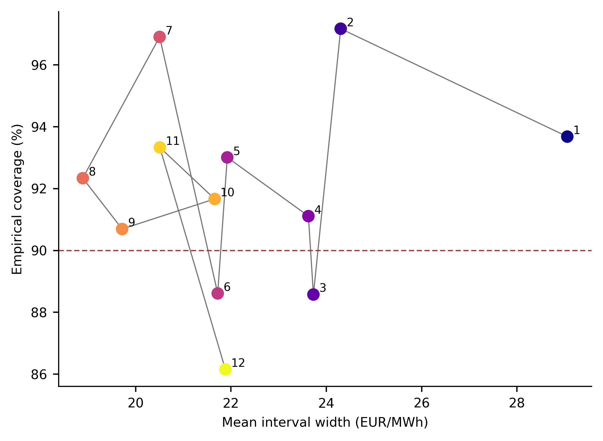
Monthly ROWCC coverage ranges from 86.16% in December to 97.17% in February, as reported in Table 3. Eight months meet or exceed the nominal 90% target by at least 0.69 percentage points, while March, June, and December fall below 90%. January intervals are widest at 29.05 EUR/MWh, followed by February at 24.30 EUR/MWh. Width declines toward late summer, reaching 18.89 EUR/MWh in August, then rises through the final quarter. The correction component follows a similar but not identical path because the raw quantile width also changes.
| Month | PICP (%) | MIW | Month | PICP (%) | MIW |
|---|---|---|---|---|---|
| Jan | 93.68 | 29.05 | Jul | 96.91 | 20.50 |
| Feb | 97.17 | 24.30 | Aug | 92.34 | 18.89 |
| Mar | 88.58 | 23.73 | Sep | 90.69 | 19.72 |
| Apr | 91.11 | 23.62 | Oct | 91.67 | 21.66 |
| May | 93.01 | 21.92 | Nov | 93.33 | 20.51 |
| Jun | 88.61 | 21.72 | Dec | 86.16 | 21.88 |
The reliability–sharpness path in Figure 5 shows that wider months are not automatically better calibrated. January is both wide and above target, whereas March has similar width but lower coverage. July combines high coverage with moderate width, and December has intermediate width but the lowest coverage. This non-monotonicity supports condition-sensitive rather than purely width-based diagnostics. Calibration quality depends on whether the score history resembles the errors that actually arrive, not merely on how broad the band is.
December undercoverage is the clearest temporal warning. The six-week half-life allows ROWCC to adapt, but a rapid shift can still arrive faster than enough relevant scores accumulate. Increasing the time-decay rate would react faster but could make corrections noisy; reducing the decay would stabilize them but preserve stale information. The result therefore argues against tuning the half-life on the same test year. A future validation study should choose half-life and similarity bandwidths using rolling pre-test folds, then confirm them on a later untouched year.
The monthly results also clarify the meaning of annual 91.91% coverage. That value does not imply a 91.91% guarantee in each month. Marginal annual calibration can coexist with local deviations. For procurement decisions concentrated in a particular season, the monthly table is more relevant than the annual average. The method improves the aggregate balance but does not eliminate the need for temporal diagnostics.
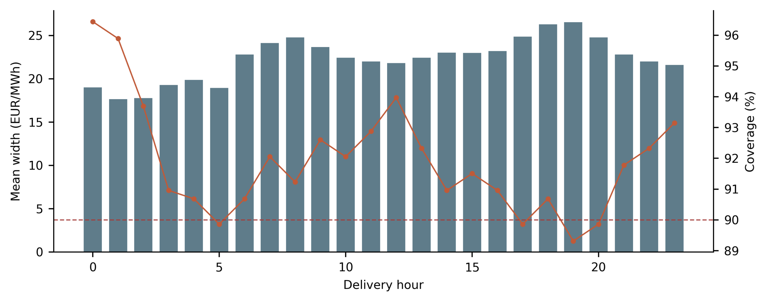
Hour-specific coverage exceeds or equals 89.0% at 20 of 24 delivery hours. The lowest values are 89.32% at 19:00 and 89.86% at 05:00, 17:00, and 20:00. Overnight coverage is generally higher, reaching 96.44% at 00:00 and 95.89% at 01:00. Mean width is smallest at 01:00, 17.66 EUR/MWh, and largest at 19:00, 26.54 EUR/MWh. The increase from early morning into the morning ramp and from late afternoon into the evening peak is economically plausible: prices become less predictable when demand and marginal generation change rapidly.
The paired bars and line in Figure 6 show that ROWCC does not obtain high overnight coverage by widening all intervals. Overnight widths are among the narrowest, yet coverage is strongest. Evening widths are broader, but coverage remains close to target rather than becoming excessive. This is the intended behavior of a heteroscedastic interval: allocate uncertainty where the conditional process is difficult rather than applying one standard error to the whole day.
The same-hour weight is central to this structure. An exact hour match receives weight one, whereas a different hour receives 0.12 before other similarity terms are applied. This ratio lets each delivery hour learn primarily from its own preceding errors but avoids a 24-way fragmentation of the calibration record. The smooth demand and volatility components provide additional transfer: an error at a neighboring high-load hour can retain meaningful influence, whereas an error from a dissimilar calm period is attenuated.
Hour-specific coverage still reveals a slight weakness near ramp periods. The intervals at 17:00–20:00 are broad, yet three of those four hours are at or just below 90%. A calibration variable measuring the slope of expected demand or the day-ahead renewable forecast might discriminate ramp conditions more directly. Such additions should be evaluated as extensions in a later study; they are not inserted post hoc here because prompt-period test outcomes must not determine new features.
Only 101 test hours meet the predetermined high-price criterion of at least 75 EUR/MWh. Raw quantile boosting covers 59.41% of them, static CQR covers 83.17%, and ROWCC covers 79.21%. All misses in this subset occur above the upper endpoint, as expected from conditioning on large realized prices. Static CQR has the best subset coverage and interval score (55.07 EUR/MWh) but a mean width of 40.14 EUR/MWh. ROWCC is narrower at 37.94 EUR/MWh, yet its interval score is higher at 58.20 EUR/MWh because several missed prices lie materially beyond the upper bound. The aggregate results and high-price results therefore rank the two calibrated methods differently.
| Method | PICP (%) | MIW (EUR/MWh) | IS (EUR/MWh) |
|---|---|---|---|
| Raw quantile boosting | 59.41 | 27.13 | 78.75 |
| Static CQR | 83.17 | 40.14 | 55.07 |
| ROWCC | 79.21 | 37.94 | 58.20 |
The diagnostic in Table 4 prevents an overly broad claim. ROWCC is best for the complete 2019 distribution under the mean interval score, but it is not best if the decision criterion is coverage exclusively during rare high prices. Recency and similarity weighting downweight distant large errors when the current state appears calmer. That behavior improves ordinary sharpness but can leave the upper endpoint vulnerable when a price jump is weakly signaled by consumption and lagged volatility. Market participants with strongly asymmetric losses may therefore prefer a one-sided upper prediction bound, an asymmetric score, or a deliberately conservative tail overlay.
The shortfall does not contradict the annual result. Standard conformal coverage is marginal over the target population, not automatically conditional on an outcome-defined tail. Conditioning on \(y_t\geq75\) selects observations after their outcomes are known and concentrates the very cases most likely to exceed an upper bound. The correct interpretation is operational: the proposed covariates and score weights do not fully identify the onset of rare price excursions. Additional pre-delivery information such as renewable production forecasts, plant unavailability, fuel prices, and cross-border constraints could improve discrimination, but their timestamp integrity must be documented carefully.
Earlier interval methods frequently train lower and upper networks through composite objectives that trade coverage against width. Lower–upper bound estimation is a prominent example [37], and related approaches have been applied to wind generation and price intervals [38], [39]. These methods can be effective, but their loss weights embed a user-selected preference and their reported aggregate coverage may not reveal time-local failures. ROWCC instead trains ordinary conditional quantiles with pinball loss and performs an explicit, inspectable calibration step. The target error rate has a direct probabilistic meaning, while the weighting function describes which past errors are treated as relevant.
The comparison with static CQR also complements recent price-forecasting studies that emphasize richer predictive distributions. A model can represent complex nonlinearities yet remain empirically miscalibrated under a new year. Calibration is therefore not a substitute for predictive structure, and predictive structure is not a substitute for calibration. The raw interval’s 76.56% coverage demonstrates the latter point; the remaining 2019 monthly and tail deviations demonstrate the former. A strong operational system needs both a conditional model that ranks uncertainty correctly and a calibration layer that adapts the level of that uncertainty.
The findings align with broader forecasting guidance that evaluation should be chronological, multimetric, and matched to the decision horizon [40]. Random cross-validation would obscure nonstationarity. Reporting only PICP would favor global CQR because it overcovers; reporting only width would favor the invalid raw interval. The interval score selects ROWCC because it balances these dimensions. Conditional tables then qualify that selection for seasonal, hourly, and tail-specific use.
The numerical comparison also clarifies how the correction changes over the year. The mean forecast-specific addition is largest in January and smallest in August. That movement is not imposed by a calendar lookup; it emerges from the weighted score archive. Large recent errors retain substantial influence through exponential decay, and same-hour observations concentrate that influence within comparable parts of the daily auction. As quieter observations accumulate, the weighted upper score quantile contracts. If larger errors recur, the quantile expands. Consequently, the calibration component can decline even when the base interval remains moderately broad, or it can expand when the base quantiles have not yet reflected a change in realized error magnitude.
This distinction explains why monthly width is not a direct proxy for the conformal correction. Total width equals the distance between the two boosted quantiles plus twice the correction. The first term represents conditional dispersion inferred from the predictor vector; the second represents empirical miscalibration among preceding comparable forecasts. January combines broad predictive quantiles with a relatively large mean correction of 5.60 EUR/MWh. August combines narrower predictive quantiles with a smaller correction of 2.93 EUR/MWh. March and December demonstrate that contraction can occasionally proceed faster than the subsequent error process warrants, which is visible in their below-target coverage.
The directional miss rates add another layer of interpretation. Raw quantile boosting misses almost equally below and above, so a symmetric correction is reasonable for the central annual objective. After calibration, lower-end misses remain more frequent than upper-end misses. This imbalance may reflect a downward change in the 2019 price distribution relative to the late-2018 calibration period, negative-price behavior, or imperfect conditional quantile estimation. A symmetric conformal score cannot correct unequal tails independently. Nevertheless, the total interval score favors ROWCC, showing that the residual asymmetry does not offset the gain in sharpness for the complete year. Applications whose financial loss is strongly one-sided should evaluate separate lower and upper scores before deployment.
Comparison with global CQR reveals when local relevance is most valuable. A constant correction preserves a memory of the largest calibration-period errors at every hour, even after many lower-error test observations have accumulated. ROWCC gradually discounts those distant events but does not discard them abruptly. Its global anchor retains a small part of the initial correction, and the nonzero similarity floors allow atypical observations to influence future forecasts. The method therefore behaves as a continuum between strict local matching and complete pooling. The annual result suggests that this compromise is better suited to the observed 2019 error sequence than either uncorrected quantiles or complete pooling.
The same evidence cautions against interpreting adaptation as automatic robustness. If an unprecedented event occurs, no weighting of prior residuals can create information that the archive does not contain. The first hours of a new disturbance can still be missed, and the high-price diagnostic confirms this vulnerability. Adaptation becomes effective only after the predictive covariates or newly observed errors signal the change. The method should therefore be viewed as a disciplined mechanism for reallocating empirical uncertainty, not as a substitute for market variables that anticipate supply scarcity or network stress.
ROWCC can be deployed as a lightweight layer around an existing quantile forecaster. Before each auction deadline, the base model produces lower, median, and upper quantiles. The calibration module compares the forthcoming delivery condition with a rolling archive of scored forecasts, calculates weights, and returns the correction. Once the delivery price is observed, the new score enters the archive. The predictive model need not be retrained hourly. This separation permits frequent uncertainty updates at lower computational cost than full model refitting.
The correction is also auditable. An analyst can inspect whether a wide interval arose from broad base quantiles, large recent conformity scores, hour matching, demand similarity, or volatility similarity. Such traceability is useful when a trading desk must explain why uncertainty changed. The procedure does not assign causal meaning to its variables: matching on consumption and volatility identifies predictive resemblance, not intervention effects. It nevertheless offers more operational detail than a single annual coverage percentage.
The measured gain is meaningful but should not be overstated. A 20.06% reduction in mean width relative to static CQR accompanies annual coverage that remains above 90%, and the interval score improves by 8.17%. These are test-year results from one national market record. They establish feasibility and motivate broader validation; they do not prove universal superiority across bidding zones, price caps, market redesigns, or energy crises.
Whether a conformal correction conditioned on both recency and operating similarity can preserve near-nominal coverage while reducing the conservatism of a single global correction. The French 2019 test answers that question affirmatively for the studied record. Raw 5–95% gradient-boosted quantiles covered only 76.56% of prices. A global split-conformal adjustment raised coverage to 95.82% but required a mean width of 27.88 EUR/MWh. ROWCC achieved 91.91% coverage with a 22.29 EUR/MWh mean width and the lowest mean interval score, 28.94 EUR/MWh. It therefore recovered most of the missing reliability while removing 20.06% of the global method’s average width.
The improvement is attributable to calibration rather than point prediction: all alternatives share a median MAE of 4.84 EUR/MWh and RMSE of 6.45 EUR/MWh. The weighted score distribution permits corrections to respond to recent errors arising at the same delivery hour and under comparable consumption and lagged-volatility conditions. Hourly diagnostics show appropriately narrow overnight bands and broader ramp-period bands, with coverage at or above 89% for 20 of 24 hours. Monthly coverage nevertheless falls to 86.16% in December, and coverage among the 101 high-price hours is 79.21%. The answer is thus precise rather than generic: operating-condition weighting improves the annual reliability–sharpness balance, but it does not fully calibrate rare upper-tail events or abrupt seasonal shifts.
For operational use, ROWCC offers a transparent uncertainty layer that can update whenever a realized price arrives without retraining the base quantile model. For research, the results identify the next decisive test: validate the same fixed procedure on later crisis periods and additional bidding zones, then assess whether point-in-time renewable, outage, fuel, and interconnection variables improve tail discrimination. Until that validation is complete, the reported intervals should be interpreted as empirically calibrated year-ahead forecasting evidence for this market record, not as a universal distribution-free guarantee under arbitrary market change.
Not applicable
The author declares no competing interests.
There is no specific funding to support this research.
The experimental data used to support the findings of this study are available from the author upon request.