
Malware classification has become a central defensive task because malicious executables increasingly combine rapid distribution, economic incentives, and code transformation techniques that weaken signature matching. Ransomware services, commodity loaders, and modular payload delivery have lowered the operational threshold for campaigns that can disrupt public services and connected infrastructure [1], [2]. Static inspection remains attractive in this environment because it can examine a file before execution and can be deployed where sandbox detonation is costly, slow, or operationally unsafe. Its weakness is equally clear: packing, encryption, polymorphism, and byte-level transformation can alter the visible representation of a program without changing its harmful purpose. The classification problem is therefore not simply to separate benign and malicious files under a fixed distribution. A defensible detector must retain useful behavior when an executable has been transformed to suppress recognizable byte patterns.
The conversion of executable bytes into images offers one response to that difficulty. A binary can be read as an ordered sequence of values from 0 to 255, arranged into a two-dimensional intensity field, and passed to a convolutional network. The operation avoids manual disassembly and permits spatial filters to detect recurring textures, transitions, and section boundaries. Early investigations showed that convolutional architectures can distinguish malware families from grayscale renderings [3]; subsequent studies expanded visual analysis with opcode information, attention, multiple views, or combined static attributes [4]–[6]. The attraction of this representation is practical as much as statistical. Mature image architectures, optimized training procedures, and readily available pretrained parameters can be reused for binary-derived inputs even though natural photographs and executable files arise from different domains.
Transfer learning reduces the amount of task-specific optimization required for deep image classifiers. General accounts distinguish feature transfer, parameter initialization, and domain adaptation according to what knowledge is retained and how the target distribution differs from the pretraining distribution [7], [8]. In malware analysis, transferred convolutional features have been used to classify visualized binaries and to recognize obfuscation variants [9], [10]. The method is not guaranteed to succeed merely because a large image network is available. Natural-image filters encode local edge and texture regularities; binary images encode byte ordering, section layout, compiler behavior, packing, and transformation artifacts. The semantic mismatch requires empirical comparison, and the comparison must cover the file conditions expected after deployment.
Residual networks and EfficientNet variants embody different architectural priorities. Residual connections support the optimization of deeper networks by allowing a block to learn a residual mapping relative to its input [11]. EfficientNet couples depth, width, and resolution through compound scaling, while EfficientNetV2 revises the operator mix to improve training speed and parameter use [12], [13]. These designs can therefore respond differently to binary textures. A compact residual network may preserve local structure efficiently; a scaled mobile-inverted bottleneck network may offer stronger feature reuse or different precision–recall behavior. Statements that one family is universally superior are consequently difficult to justify without specifying both the file condition and the operational preference.
Obfuscation sharpens this selection problem. XOR transformation changes byte values systematically, while Shikata Ga Nai combines polymorphic XOR additive feedback with code mutation, producing different outputs across applications. XOR-based adversarial modification has been shown to evade detectors even when the underlying malicious functionality is retained [14]. Entropy can help identify packing or encryption because transformed regions often display altered byte-frequency distributions [15], [16], but entropy alone cannot determine malicious intent. A staged detector may first assess whether transformation is likely and then route the file to a classifier trained for the appropriate condition. The scheme used in each route still needs to be selected, and that decision must account for false alarms as well as missed malware.
The usual selection procedure ranks architectures by accuracy or F1. Accuracy summarizes the fraction of correct decisions, but it can obscure asymmetric error costs and class imbalance. Precision describes the reliability of positive alarms, recall describes the fraction of malicious files detected, and F1 balances precision with recall through their harmonic mean. These quantities are related but not interchangeable. A security operations center with expensive manual investigation may emphasize precision; a critical endpoint may emphasize recall; a mixed deployment may require a stable compromise. Selecting on one quantity silently fixes an operational preference even when that preference has not been stated.
Condition aggregation creates a second silent choice. Averaging unobfuscated and obfuscated values assumes equal importance and allows a high clean-file value to compensate for weaker transformed-file behavior. Taking the minimum is conservative but may be controlled by a single precision value. Choosing the obfuscated condition alone may be appropriate under a high-risk threat model but ignores common benign and ordinary malicious files. An effective comparison should therefore expose at least three aspects: coordinatewise superiority, protection of the weakest coordinate, and sensitivity to unknown importance weights. These aspects answer different questions and should not be collapsed prematurely.
Machine-learning evaluation in security is especially vulnerable to hidden design choices. Temporal leakage, family overlap, sampling artifacts, and unrealistic train–test construction can inflate apparent success [17], [18]. Guidance for security learning studies consequently emphasizes explicit threat assumptions, careful separation, and interpretation tied to deployment decisions [19]. Public collections and challenges such as EMBER, the Microsoft Malware Classification Challenge, and BODMAS have improved access to labeled executable material and temporally organized static attributes [20]–[22]. Even with strong collections, however, model selection remains a separate inferential act. A sound file split does not determine whether a one-hundredth percentage-point lead is decisive, nor whether a lead survives a different weighting of error-related quantities.
Malware defense also operates within a connected system rather than at an isolated classifier. Vision transformers and feature-fusion networks have been applied to anomalous traffic, demonstrating that visual learning principles can extend from binary files to communication behavior [23]. Compartmental models of malware propagation similarly show that detection delay and transmission processes jointly determine campaign scale [24]. These studies motivate a broader interpretation of classification errors. A false negative can allow propagation to continue, whereas a false positive can interrupt a legitimate process or impose analyst work. The appropriate error preference depends on where the classifier is placed, what secondary inspection follows, and whether an automated action is reversible.
Recent malware classifiers illustrate the diversity of available evidence. Header embeddings combine compact byte regions with neural or clustering procedures [25]. Opcode-category representations can yield low-dimensional descriptions that remain effective across malware families [26], while sequential opcode embeddings attempt to preserve local program regularities [27]. End-to-end byte models remove handcrafted feature extraction by applying convolutions directly to long executable sequences [28]. Attention mechanisms and depth-wise convolution have also been examined for virtual-machine-obfuscated material [29], and dynamic traces have been combined with explainable deep learning for mobile malware [30]. These approaches differ in representation, execution requirements, and susceptibility to transformation. Their variety reinforces the need for selection rules that state what is valued rather than presenting a single leader without qualification.
The present study addresses the following research question: among ResNet18, ResNet34, EfficientNetB3, and EfficientNetV2S, which network offers the strongest and most preference-stable classification choice when four performance quantities are considered simultaneously across unobfuscated and obfuscated binaries? The question differs from asking which network has the largest F1 value in either condition. It requires a decision that remains interpretable when the relative importance of accuracy, precision, recall, and F1 is unknown.
The contribution is a condition-stratified analysis built from an eight-coordinate Structural matrix. First, coordinatewise comparisons identify strict dominance and local trade-offs without imposing weights. Second, an arithmetic aggregate, a harmonic aggregate, a minimum-coordinate floor, dispersion, and mean condition loss describe central performance and resistance to obfuscation. Third, one million weight vectors are drawn uniformly from the probability simplex to estimate the portion of admissible preference space in which each architecture ranks first. The resulting decision is conditional rather than absolute: ResNet18 is identified as the stable general choice, while EfficientNetB3 occupies a small but explainable region associated with unusually strong emphasis on obfuscated-file precision. This distinction is important because a small preference region is not equivalent to no defensible region.
The paper is organized as follows. Section II defines the analytical matrix and the condition-stratified decision procedure. Section III presents and interprets the numerical findings, including every figure and table. Section IV states the boundaries of the claims. Section V answers the research question and gives the resulting deployment rule.
The analysis uses four convolutional backbones evaluated in two binary conditions. ResNet18 and ResNet34 represent compact and deeper residual networks. EfficientNetB3 represents compound-scaled mobile inverted bottlenecks, and EfficientNetV2S combines fused and mobile inverted bottleneck operators. The unobfuscated condition contains executable images produced without XOR or Shikata Ga Nai. The obfuscated condition combines binaries transformed with those two encoders. For each architecture and condition, accuracy, precision, recall, and F1 are expressed as percentages.
The 32 values in Table 1 were assembled from the numerical evaluation of 15,628 benign files and 15,821 malicious files per encoding conditiono [31]. No sample-level prediction vector is assumed, and no confidence interval is reconstructed from rounded percentages. The unit of analysis is an architecture–condition–quantity coordinate, not an individual executable.
| Network | Binary condition | Accuracy | Precision | Recall | F1 |
|---|---|---|---|---|---|
| ResNet18 | Unobfuscated | 99.34 | 99.52 | 99.16 | 99.34 |
| ResNet18 | Obfuscated | 97.42 | 95.65 | 99.43 | 97.50 |
| ResNet34 | Unobfuscated | 99.26 | 99.48 | 99.03 | 99.26 |
| ResNet34 | Obfuscated | 97.39 | 95.60 | 99.40 | 97.46 |
| EfficientNetB3 | Unobfuscated | 98.96 | 98.99 | 98.96 | 98.98 |
| EfficientNetB3 | Obfuscated | 97.41 | 95.72 | 99.34 | 97.49 |
| EfficientNetV2S | Unobfuscated | 99.22 | 99.53 | 98.93 | 99.23 |
| EfficientNetV2S | Obfuscated | 97.21 | 95.25 | 99.43 | 97.30 |
The matrix shows why a single-value choice is insufficient. ResNet18 has the largest clean accuracy and clean F1, EfficientNetV2S has the largest clean precision, EfficientNetB3 has the largest obfuscated precision, and ResNet18 shares the largest obfuscated recall with EfficientNetV2S. The differences are numerically small, but their direction changes with the selected coordinate. Any unconditional ranking must therefore be justified by more than the maximum entry in one column.
Let \(x_{a r q}\) denote the percentage for architecture \(a\), binary condition \(r\in\{u,o\}\), and quantity \(q\in\{A,P,R,F\}\), corresponding to accuracy, precision, recall, and F1. Each architecture is represented by an eight-dimensional vector
Architecture \(a\) strictly dominates architecture \(b\) when \(x_{a r q}>x_{b r q}\) for every coordinate. Weak dominance permits equality in at least one coordinate provided that \(a\) is never smaller and is strictly larger somewhere. For non-dominating pairs, the ordinal margin is
where a win contributes \(+1\), a loss contributes \(-1\), and a tie contributes zero. This operation retains the direction of each comparison and makes no assumption about whether a 0.01-point advantage in precision has the same operational value as a 0.01-point advantage in recall.
The dominance operation supplies the strongest available conclusion when it applies. If one architecture is no worse on every coordinate, nonnegative weighting cannot reverse its position. When dominance does not apply, the margin reveals how widely an advantage is distributed, while the subsequent weighting analysis identifies how concentrated preferences must become to reverse the overall leader.
Five summaries are calculated for every architecture. The arithmetic mean
describes equally weighted central performance. The harmonic mean
penalizes lower coordinates more strongly and is suitable when weak dimensions should not be freely compensated by high ones. Because all entries lie near 100%, the arithmetic and harmonic values are expected to be close; their ordering is nevertheless useful as a check that the conclusion does not depend on a single averaging form.
The performance floor is \(F_a^{\min}=\min_{r,q}x_{arq}\). It answers a deliberately conservative question: what is the lowest value observed for the architecture across the two conditions and four quantities? The population standard deviation
describes within-architecture dispersion across coordinates. A lower value means greater numerical evenness, not necessarily better classification. Finally, mean condition loss is
Positive \(L_a\) indicates that the average unobfuscated value exceeds the average obfuscated value. This quantity does not treat an increase in recall under obfuscation as automatically favorable without context; it simply records the signed change and averages it with the other three changes. The component changes remain visible in the complete matrix.
These summaries are interpreted jointly. A high arithmetic mean supports broad overall performance, a high harmonic mean resists compensation, a high floor protects the weakest coordinate, a small dispersion indicates balance, and a small condition loss indicates resistance to binary transformation. No new classifier is trained, and no latent sample-level uncertainty is claimed from the rounded entries.
Unknown operational priorities are represented by a nonnegative weight vector \(\mathbf{w}=(w_1,\ldots,w_8)\) satisfying \(\sum_j w_j=1\). For any admissible vector, architecture \(a\) receives the linear utility
The first-ranked architecture is \(a^*(\mathbf{w})=\arg\max_a U_a(\mathbf{w})\). Linear utility is used because it has an exact operational interpretation: each weight states the fraction of total decision importance assigned to one condition–quantity coordinate. It also preserves dominance. If an architecture is never worse and is better somewhere, no admissible weight vector with positive mass on that advantage can place the dominated architecture above it.
To measure selection stability, \(N=1{,}000{,}000\) independent weight vectors are drawn from a Dirichlet distribution with concentration parameters \((1,1,1,1,1,1,1,1)\). This distribution is uniform over the seven-dimensional simplex and does not privilege a criterion, a condition, or a sparse weighting pattern. The selection share is
The fixed random seed 20260827 makes the numerical integration repeatable from the included script. The Monte Carlo standard error for a share \(p\) is \(\sqrt{p(1-p)/N}\); for \(p=0.000231\), it is approximately 0.0000152 in probability units, or 0.00152 percentage points. This calculation describes numerical integration uncertainty, not uncertainty about future files.
The preference-space operation does not assert that real organizations choose weights uniformly. Its purpose is geometric: it estimates how much of the unconstrained weight simplex supports each architecture. A very small share means that a reversal requires a concentrated and unusual importance pattern. A zero share can result either from dominance or from an empty winning region under the linear rule. The pairwise operation is therefore retained to distinguish these cases.
The global weighting analysis is supplemented with a local view of obfuscated precision and recall. This pair is operationally important because it separates alarm trustworthiness from malicious-file capture. Let \(p_a=x_{aoP}\) and \(r_a=x_{aoR}\). Architecture \(a\) lies on the local Pareto frontier if no other architecture has both \(p\ge p_a\) and \(r\ge r_a\), with at least one strict inequality. Accuracy and F1 are then consulted to resolve points that remain on the local frontier. This sequence prevents a two-coordinate plot from being mistaken for the complete eight-coordinate decision.
The complete performance field in Figure 1 reveals two regularities. First, all networks remain above 97.21% in accuracy and above 97.30% in F1 across both conditions, indicating that the choice concerns refinement among strong classifiers rather than separation of an acceptable system from a failed one. Second, precision experiences the largest decline after obfuscation. Unobfuscated precision ranges from 98.99% to 99.53%, whereas obfuscated precision ranges from 95.25% to 95.72%. Recall behaves differently: every obfuscated recall exceeds the corresponding unobfuscated recall. The transformed-file condition therefore shifts the error balance toward capturing more malware at the cost of more benign files being classified as malicious.
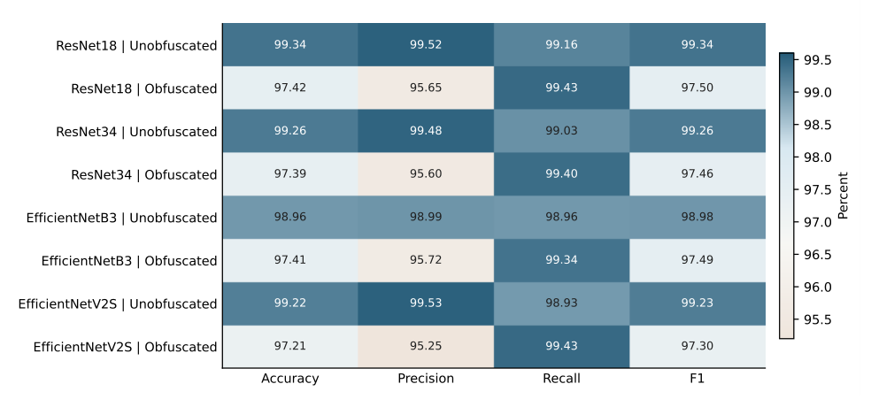
This error redistribution matters more than the narrow differences among network families. A detector with 99.43% recall but 95.65% precision will miss relatively few malicious files, yet its positive queue contains more benign files than the clean-file precision suggests. In a high-volume endpoint service, even a fraction of a percentage point can change analyst workload. Conversely, lower precision may be acceptable when the cost of a missed malicious executable greatly exceeds the cost of a false alarm. The heat map thus supports a conditional choice: the architecture ranking should not be separated from the intended error cost.
ResNet18 occupies the most consistently dark cells in the full field. It leads clean accuracy, clean recall, clean F1, obfuscated accuracy, and obfuscated F1; it also shares the obfuscated recall lead. Its two losses are narrowly defined. EfficientNetV2S exceeds it in clean precision by 0.01 percentage points, and EfficientNetB3 exceeds it in obfuscated precision by 0.07 points. Neither competitor converts that local gain into a higher F1 or accuracy. The balance between precision and recall therefore favors ResNet18 unless precision receives disproportionate importance.
The F1 transition in Figure 2 shows that all four networks lose between 1.49 and 1.84 percentage points when moving from unobfuscated to obfuscated files. The lines converge near 97.5%, so the broader clean-file spread contracts under transformation. ResNet18 falls from 99.34% to 97.50%, ResNet34 from 99.26% to 97.46%, EfficientNetB3 from 98.98% to 97.49%, and EfficientNetV2S from 99.23% to 97.30%.
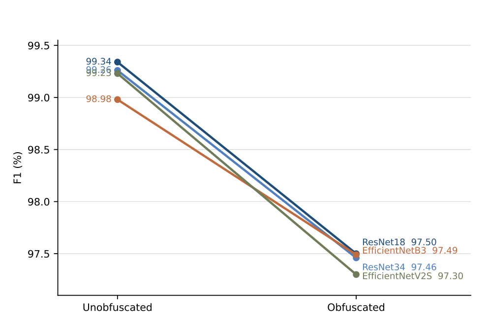
The transition alters the practical interpretation of the leaders. ResNet18 has the highest value at both endpoints, but EfficientNetB3 preserves F1 most strongly: its decline is 1.49 points, compared with 1.84 for ResNet18. EfficientNetB3 nearly closes a 0.36-point clean-file deficit and finishes only 0.01 point behind. This pattern is consistent with a representation that sacrifices some clean-file discrimination while remaining less sensitive to transformation. It does not establish a causal architectural mechanism because activations and sample-level errors are unavailable, but it identifies a precise empirical property that can guide a follow-up study.
The smallest transition alone would select EfficientNetB3, yet that choice would reward preservation without considering starting level. A system could have a small decline because its clean performance is already lower. The summaries in Table 2 prevent that interpretation by presenting absolute central values, the weakest coordinate, and the decline together.
| Architecture | Arithmetic mean | Harmonic mean | Minimum | Std. dev. | Clean mean | Obfuscated mean | Mean loss |
|---|---|---|---|---|---|---|---|
| ResNet18 | 98.4200 | 98.4020 | 95.6500 | 1.3224 | 99.3400 | 97.5000 | 1.8400 |
| ResNet34 | 98.3600 | 98.3423 | 95.6000 | 1.3121 | 99.2575 | 97.4625 | 1.7950 |
| EfficientNetB3 | 98.2313 | 98.2171 | 95.7200 | 1.1704 | 98.9725 | 97.4900 | 1.4825 |
| EfficientNetV2S | 98.2625 | 98.2414 | 95.2500 | 1.4308 | 99.2275 | 97.2975 | 1.9300 |
The tabulated summaries yield three different leaders. ResNet18 leads both averages, with an arithmetic mean of 98.4200% and a harmonic mean of 98.4020%. EfficientNetB3 has the highest minimum at 95.72%, the smallest dispersion at 1.1704 points, and the smallest mean condition loss at 1.4825 points. EfficientNetV2S has neither the highest central value nor the strongest floor; its 95.25% obfuscated precision sets the lowest floor and its 1.93-point mean decline is the largest. ResNet34 is close to ResNet18 but never exceeds it on an individual coordinate.
The near agreement of the arithmetic and harmonic orderings is informative. Because the harmonic mean penalizes lower coordinates, a reversal would have indicated that the arithmetic leader depended on compensation from very high values. No reversal occurs: ResNet18 remains first, ResNet34 second, EfficientNetV2S third, and EfficientNetB3 fourth by the harmonic aggregate. EfficientNetB3’s superior floor does not overcome its lower clean-file values under equal treatment of all coordinates. The distinction between mean leadership and floor leadership is therefore genuine rather than an artifact of the averaging formula.
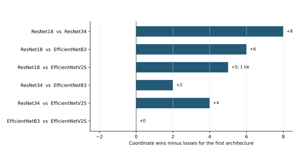
Pairwise comparisons in Table 3 establish which rankings are weight-independent. ResNet18 defeats ResNet34 on all eight coordinates, giving a margin of \(+8\). Consequently, ResNet34 cannot outrank ResNet18 under any nonnegative weighting of these coordinates. ResNet18 wins seven coordinates and loses one against EfficientNetB3, producing a margin of \(+6\). Against EfficientNetV2S, it wins six, loses one, and ties one, producing \(+5\). The tie is obfuscated recall at 99.43%.
These counts clarify why a tiny numerical lead can still matter. EfficientNetB3 is not dominated by ResNet18 because its obfuscated precision is higher. EfficientNetV2S is not dominated by ResNet18 because its clean precision is higher and its obfuscated recall is tied. Their potential preference regions are nevertheless constrained by losses on most other coordinates. EfficientNetB3 and EfficientNetV2S split their comparison four to four, but their mean difference favors EfficientNetV2S by 0.03125 percentage points. The equal ordinal count and unequal average difference show why both direction and magnitude are needed.
The graphical margins in Figure 3 make the hierarchy visible without introducing a composite score. ResNet18 has broad directional support against every competitor. ResNet34’s positive margins over both EfficientNet variants do not make it selectable because it is strictly dominated by ResNet18. EfficientNetB3’s zero margin against EfficientNetV2S conceals an important condition pattern: B3 is stronger in the obfuscated condition, while V2S draws much of its advantage from unobfuscated precision and related clean values. For deployments explicitly centered on transformed binaries, B3 is therefore the more relevant EfficientNet variant.
| Pair | Wins | Losses | Ties | Margin |
|---|---|---|---|---|
| R18–R34 | 8 | 0 | 0 | +8 |
| R18–E-B3 | 7 | 1 | 0 | +6 |
| R18–E-V2S | 6 | 1 | 1 | +5 |
| R34–E-B3 | 5 | 3 | 0 | +2 |
| R34–E-V2S | 6 | 2 | 0 | +4 |
| E-B3–E-V2S | 4 | 4 | 0 | 0 |
This finding also cautions against choosing a deeper member of an architecture family solely because it has more layers. ResNet34 loses to ResNet18 on every observed coordinate. Residual depth can increase representational capacity, but the binary-image task may not benefit from that additional capacity under the available training procedure. Similar cautions apply to compound scaling. The theoretical ability to scale width, depth, and resolution efficiently does not guarantee a better position when the target textures differ substantially from natural images.
The robustness map in Figure 4 places the weakest coordinate on the vertical axis and mean condition loss on the horizontal axis. The desirable direction is upward and leftward: a point should protect its weakest value while changing little after obfuscation. EfficientNetB3 occupies that corner, with a 95.72% floor and a 1.4825-point mean loss. ResNet18 lies higher than the other residual network but farther right, reflecting its stronger absolute values and larger clean-to-obfuscated decline. EfficientNetV2S is inferior on both displayed dimensions to each of the other three architectures.
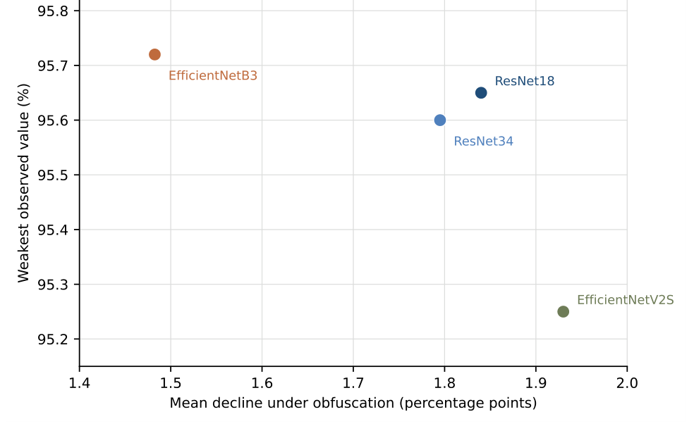
The map identifies a deployment rule that an overall mean cannot express. If the institution defines robustness as maximizing the lowest observed percentage while minimizing average transformation loss, EfficientNetB3 is the appropriate choice. If robustness means maintaining the highest combined accuracy, precision, recall, and F1 across both conditions, ResNet18 remains appropriate. Neither definition is intrinsically correct; the choice depends on whether low-tail protection or total performance receives priority.
The map also shows that ResNet34 offers no useful compromise. It has a lower floor than ResNet18, only a slightly smaller condition loss, and lower values on all eight coordinates. EfficientNetV2S similarly provides no floor-loss advantage. Removing these dominated or unattractive options simplifies operational consideration to a two-architecture question: broad superiority with ResNet18 or transformed-file floor protection with EfficientNetB3.
The preference-space integration produces the strongest evidence for the general choice. ResNet18 ranks first for 999,769 of the one million sampled weight vectors, corresponding to 99.9769%. EfficientNetB3 ranks first for 231 vectors, corresponding to 0.0231%. ResNet34 and EfficientNetV2S never rank first. The shares and Monte Carlo standard errors are shown in Table4.
| Network | Share (%) | MC error (pp) |
|---|---|---|
| ResNet18 | 99.9769 | 0.00152 |
| ResNet34 | 0.0000 | 0.00000 |
| EfficientNetB3 | 0.0231 | 0.00152 |
| EfficientNetV2S | 0.0000 | 0.00000 |
The numerical integration error is small relative to the difference between the two nonzero shares. More importantly, the result has a geometric explanation. EfficientNetB3 can win only by placing very large weight on obfuscated precision, its sole advantage over ResNet18, while assigning little weight to the seven coordinates on which it loses. ResNet18 wins throughout nearly the entire simplex because its advantages are distributed broadly. The result is thus not a fragile artifact of equal weighting.
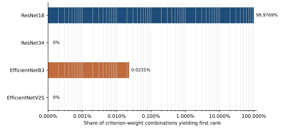
The logarithmic display in Figure 5 preserves the small EfficientNetB3 region that would disappear on a linear axis. Showing that region is scientifically important. Reporting only that ResNet18 wins almost always would hide the exact circumstance in which another architecture is rational. At the same time, the 0.0231% share prevents the local precision advantage from being overstated. An organization should choose EfficientNetB3 on preference grounds only if it can articulate why obfuscated precision overwhelms clean accuracy, clean precision, clean recall, clean F1, obfuscated accuracy, obfuscated recall, and obfuscated F1 together.
ResNet34’s zero share follows directly from strict dominance. EfficientNetV2S is not strictly dominated by ResNet18 because of its 0.01-point clean precision advantage and tied obfuscated recall, yet it still has no winning region in the sampled simplex. Its disadvantages elsewhere are too large for those coordinates to establish a higher linear utility. The distinction between mathematical impossibility and numerically empty preference space should be retained: the former applies to ResNet34; the latter characterizes EfficientNetV2S under this integration.
The small EfficientNetB3 region can be understood without relying solely on Monte Carlo counts. Subtracting the ResNet18 vector from the EfficientNetB3 vector gives
where the coordinates follow the order defined in Section II. EfficientNetB3 therefore outranks ResNet18 only when the positive term \(0.07w_{oP}\) exceeds the sum of seven weighted deficits. In explicit form,
This inequality demands a weight concentrated near obfuscated precision. Even modest importance on unobfuscated precision is costly to B3 because its deficit on that coordinate is 0.53 points, more than seven times its obfuscated-precision advantage. The analytical inequality and the simulated share therefore tell the same story using different forms of evidence.
EfficientNetV2S faces an even narrower route to first place. Relative to ResNet18, its only strict advantage is 0.01 point in unobfuscated precision, while its deficits include 0.40 point in obfuscated precision, 0.23 in unobfuscated recall, and 0.21 in obfuscated accuracy. A weight vector placed exactly on clean precision would select EfficientNetV2S, but the surrounding winning neighborhood is extremely small. None of the one million uniform draws entered it. This observation prevents an incorrect statement that the network can never win; instead, it shows that winning requires a practically singular preference. The difference between a boundary-centered possibility and a preference region with measurable volume is central to weight-stability analysis.
The integration also reveals why equal weighting is useful but incomplete. Equal weights select ResNet18 because its arithmetic mean is largest. The simplex calculation asks whether that decision remains after equal weighting is relaxed in every direction at once. A 99.9769% share confirms that it does. If the share had been close to 50%, the equal-weight selection would have been fragile even if its mean were highest. Weight-space volume thus supplies information that a point estimate cannot provide.
The local frontier in Figure 6 isolates the operational tension behind the small EfficientNetB3 region. B3 has the highest obfuscated precision at 95.72%, but the lowest obfuscated recall at 99.34%. ResNet18 has 95.65% precision and 99.43% recall. The 0.07-point precision gain is accompanied by a 0.09-point recall loss. ResNet34 is locally dominated by ResNet18, and EfficientNetV2S has the same recall as ResNet18 but lower precision.
The local trade-off can be expressed through an alarm-cost interpretation. Higher precision reduces the proportion of benign files among positive alarms, which may save analyst time or prevent unnecessary quarantine. Higher recall reduces the proportion of malicious files that pass undetected. EfficientNetB3 is favored when the marginal cost of an additional false alarm substantially exceeds the marginal cost of an additional missed malicious file, after accounting for prevalence and downstream controls. In most security contexts the opposite relation is common, which strengthens the case for ResNet18, but the cost relation should be stated rather than assumed.
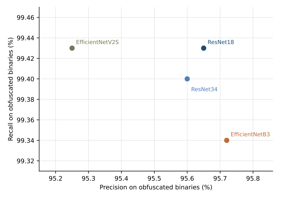
Accuracy and F1 resolve the local frontier in favor of ResNet18 under balanced concern. On obfuscated files, ResNet18 has 97.42% accuracy compared with 97.41% for EfficientNetB3, and 97.50% F1 compared with 97.49%. These 0.01-point differences are too small to justify claims of large practical superiority, yet their direction agrees with the seven-coordinate dominance pattern. The conclusion is therefore based on consistency across quantities and weight space, not on treating hundredths of a percentage point as independently decisive.
The operational effect of the precision difference depends on prevalence. Precision is not an intrinsic false-alarm rate; it is the proportion of positive decisions that are truly malicious and therefore changes with the mixture of benign and malicious files. If deployment prevalence differs from the balanced evaluation collection, the observed precision values will not transfer unchanged even when sensitivity and specificity remain stable. The choice between 95.65% and 95.72% should consequently be revisited with local prevalence or with confusion counts from a representative stream. The current comparison establishes which architecture had the stronger positive predictive value in the evaluated transformed-file mixture.
Recall has a more direct conditional meaning: among malicious files, it records the detected fraction. The 0.09-point recall difference between ResNet18 and EfficientNetB3 corresponds to nine additional detected files per 10,000 malicious files if the percentages transfer exactly. The 0.07-point precision difference cannot be translated into a fixed number of saved false alarms without knowing the number of positive decisions and the operational prevalence. This asymmetry often makes recall differences easier to communicate but does not make precision less important.
Threshold selection may also move both points. Neural classifiers emit continuous scores that are converted into labels at a chosen threshold. A higher threshold commonly raises precision and lowers recall, meaning that an architecture with lower precision at one threshold may match a competitor after calibration. A complete deployment comparison should therefore examine precision–recall curves, calibration error, and decision cost across thresholds. The present point comparison remains valuable because it evaluates the published operating points, but it should not be interpreted as the entire attainable frontier of either network.
Calibration is particularly relevant when an entropy stage routes a file before classification. Routing error changes the distribution seen by each classifier, and score calibration obtained on correctly routed validation files may not hold for misrouted files. A deployment should preserve route labels, classifier scores, and final decisions so that error sources can be separated. Without that separation, a change in positive predictive value might be attributed to the backbone when it actually arises from the obfuscation decision.
The eight coordinates describe two linked error geometries. In the unobfuscated condition, all architectures have precision and recall near 99%, and the choice is mainly a refinement of already balanced behavior. In the obfuscated condition, recall is consistently above 99.3% while precision is below 95.8%. The classifier is therefore positioned toward aggressive malicious-file capture. F1 falls because the precision decline is much larger than the recall increase.
This geometry has consequences for automated actions. When a positive classification triggers immediate quarantine, a benign false alarm can stop a legitimate service, remove a trusted executable, or generate user support cost. Higher precision then has tangible value. When a positive classification initiates a secondary sandbox or human review, the first-stage false alarm is less damaging, and higher recall may be preferable. A detector cannot be selected responsibly without identifying which downstream action follows its output.
The strong transformed-file recall may also produce a misleading sense of safety if families are unevenly distributed. An aggregate recall of 99.43% can coexist with weaker behavior for a rare family or for a particular encoder. Family-stratified confusion counts would allow a worst-family floor analogous to the coordinate floor used here. Such reporting is especially important when the malicious collection contains many variants from a few families. The present conclusion concerns aggregate malicious-file capture only.
False positives deserve equally careful stratification. System binaries, signed utilities, installers, and compressed benign applications can exhibit different byte textures. An obfuscation procedure applied uniformly to benign files may not reflect the transformations used by legitimate software vendors. Precision on transformed benign files should therefore be examined by software category and signing status. EfficientNetB3’s small precision advantage may be concentrated in one benign category or spread evenly; the aggregate value cannot distinguish these possibilities.
The network decision should consequently be paired with monitoring quantities that are not part of training. Useful operational observations include positive volume per endpoint, analyst confirmation rate, quarantine reversals, family-specific misses, route errors, and score drift over time. These observations connect statistical performance to defensive workload. They also provide evidence for revisiting the weight vector when organizational costs change.
The selection result complements several strands of malware research. Direct byte models such as MalConv demonstrate that raw executables can be processed without two-dimensional rendering [28], while image classifiers show that byte textures remain discriminative [3]. Header and opcode methods use more semantically localized information [25]–[27]. Visual transfer learning offers fast adaptation but inherits a domain mismatch from natural images. The present findings suggest that compact residual features provide the strongest average choice for the evaluated binary images, while compound-scaled features preserve a slightly better precision floor under obfuscation.
The improvement in obfuscated recall for every network deserves particular attention. A transformation that raises recall while lowering precision may change image regularities in a way that makes malicious examples easier to capture but reduces class separation for benign transformed files. Similar behavior can occur when a classifier learns transformation artifacts rather than program semantics. Obfuscation detection studies on Android applications and virtualized code have emphasized the need to separate recognition of transformation from recognition of maliciousness [29], [32]. The present matrix cannot determine whether transformation artifacts drive the change, but the consistent direction across architectures makes this a testable hypothesis.
Adversarial malware work further cautions that high values on known transformations do not establish resistance to adaptive evasion. Transferred generative models and byte-level perturbations can create evasive files while preserving behavior [33], [34]. Robustness to XOR and Shikata Ga Nai should consequently be described by those named conditions, not generalized to all packing, encryption, or semantic-preserving attacks. The weight-stable architecture choice answers a decision question within the available conditions; it does not certify adversarial security.
Temporal and family-aware validation remain essential. Collections can become stale as malware families, compilers, and packers evolve [17]. Temporal evaluation has shown that apparent performance can change substantially when training and testing respect chronological order [18]. Windows collections from the Microsoft classification challenge and BODMAS support family-aware and temporal investigation [21], [22]. Applying the same condition-stratified selection method to time-separated predictions would reveal whether ResNet18’s weight stability persists under distribution drift.
Model efficiency is another relevant consideration, although it is not included in the eight-coordinate utility because exact common-unit latency, energy, and memory values are not available in the matrix. Compact residual networks are often attractive when inference must occur close to endpoints. EfficientNet was explicitly designed to improve accuracy–efficiency trade-offs through compound scaling [12], and EfficientNetV2 sought faster training with progressive learning and fused operators [13]. A future decision matrix should include measured latency, peak memory, energy per file, and calibration under the intended hardware. Adding those quantities could enlarge the preference region of an architecture that is slightly weaker in classification but materially cheaper to operate.
Hyperparameter choice can also alter close rankings. Cyclical learning rates and one-cycle schedules can change convergence behavior [35], while automated search methods such as tree-structured Parzen estimation and gradient-boosted decision trees can optimize discrete and continuous choices efficiently [36], [37]. When architecture differences are only 0.01 to 0.2 points, equal search budgets and identical stopping rules are necessary. Random forests and other classical learners remain useful comparators for compact static attributes [38]; they can reveal whether deep visual features justify their additional complexity.
The broader lesson is methodological. Security learning papers often emphasize the largest score, yet deployment choices involve multiple errors, conditions, and resource constraints. Surveys of deep malware detection and recent deep classifiers document rapid model development [39], [40], but ranking stability receives less attention than predictive performance. A weight-space statement makes the hidden preference explicit. It can be reported alongside ordinary values without changing the classifier or claiming a new detection mechanism.
The analysis suggests several concrete reporting practices for future malware studies. Performance tables should retain condition-specific values rather than publishing only a pooled result. Pooling can conceal that transformed-file precision is the weakest coordinate for every architecture. Separate rows also make it possible to calculate condition loss and to discover whether a network preserves performance or merely begins from a lower clean value.
Every network comparison should state a primary selection rule before inspecting the test set. If F1 is primary, the rationale should connect F1 to error cost. If several quantities matter, equal weighting may be declared, followed by a sensitivity analysis over alternative weights. Predeclaring the rule reduces the temptation to choose whichever quantity produces the preferred model. The complete table should still be published so readers can apply a different operational preference.
Rounded percentages should be accompanied by confusion counts. Counts permit exact recalculation, prevalence adjustment, paired comparison when prediction identities are available, and practical translation into missed or falsely blocked files. They also reveal whether a displayed 0.01-point difference is one file or several files. In the present matrix, rounding prevents that determination, so the conclusion relies on directional consistency rather than formal significance.
Repeated training seeds are necessary when differences are narrow. Weight initialization, augmentation order, and learning-rate schedules can shift results. A mean and interval across seeds would allow the network-selection uncertainty to be separated from preference uncertainty. The first concerns whether the performance vector itself is stable; the second concerns whether the preferred architecture is stable given a fixed vector. These are distinct questions and should be analyzed separately.
Resource observations should be measured under a common device, batch size, precision mode, and input resolution. Latency per file, throughput, peak resident memory, accelerator memory, and energy should be reported with the classification quantities. A compact model may become preferable even if its F1 is slightly lower when endpoint constraints are binding. Conversely, a server-side service may value detection more than a modest inference difference. Adding resource coordinates to the same weight-space procedure would preserve transparency.
Finally, transformed-file evaluation should name every encoder, packer, and parameter setting. A pooled “obfuscated” label is too broad for security claims. Separate XOR and Shikata Ga Nai rows would reveal whether the current B3 stability is driven by one transformation. Additional rows for packing, encryption, virtualization, dead-code insertion, section reordering, and adaptive byte modification would extend the decision matrix without changing the analytical logic. The architecture selected for one transformation family should not be presented as universally resistant.
The results support a concise two-stage selection rule. ResNet18 should be selected when the deployment assigns nonnegative, reasonably distributed importance to accuracy, precision, recall, and F1 across unobfuscated and obfuscated binaries. This recommendation is supported by the highest arithmetic and harmonic means, broad pairwise superiority, and a 99.9769% preference-space share. EfficientNetB3 should be selected only when the organization explicitly prioritizes obfuscated-file precision, the highest minimum coordinate, or the smallest mean decline under transformation strongly enough to accept lower values elsewhere.
The rule should be documented with the actual cost rationale. For example, a service that automatically blocks every positive classification may experience substantial cost from false positives and may prefer B3’s 0.07-point precision advantage. A triage service that sends positives to a secondary analyzer may care more about recall and prefer ResNet18. The architecture choice becomes auditable when the error pathway is stated in these terms.
No evidence supports choosing ResNet34 from the present matrix because it is strictly dominated by ResNet18. EfficientNetV2S likewise lacks a first-rank region under the sampled weights and has the weakest floor. These conclusions may change if memory, latency, calibration, or architecture-specific maintenance cost is introduced, but they do not change under any reweighting limited to the eight included percentages for ResNet34.
Several boundaries constrain interpretation. First, the matrix contains rounded aggregate percentages rather than individual predictions. It cannot support paired significance tests, confidence intervals for model differences, calibration analysis, or family-specific error estimates. The one-million-vector calculation measures preference geometry conditional on the matrix; it does not create additional malware observations.
Second, the obfuscated condition combines XOR and Shikata Ga Nai. Separate architecture values for the two encoders would permit a twelve-coordinate comparison and could reveal an architecture–encoder interaction. The combined values support a conclusion about the joint transformed condition only. They do not establish equal behavior for XOR, Shikata Ga Nai, commercial packers, custom encryption, virtualization, or adversarial byte insertion.
Third, accuracy, precision, recall, and F1 are statistically dependent because they arise from the same confusion counts. Treating them as separate decision coordinates is intentional: they represent distinct operational views. It should not be interpreted as eight independent observations. Preference weights express decision importance, not statistical independence.
Fourth, the uniform Dirichlet distribution is a neutral geometric device, not a survey of security practitioners. Organizations may place structured constraints on weights, such as assigning at least half of total importance to obfuscated files or twice as much importance to recall as precision. The included program can evaluate such constrained weight regions. The very large ResNet18 share indicates stability under unconstrained preferences, while a deployment-specific analysis should use documented priorities.
Fifth, the file collection is limited to x86 executables and the named benign and malicious sources used to produce the published values. Results may differ for ARM binaries, scripts, documents, mobile packages, or files collected in a later period. Malware evaluation guidance warns that temporal, family, and collection artifacts can alter apparent performance [19]. External validation should therefore preserve chronology, deduplicate related samples, and report family-aware splits.
Finally, ImageNet initialization and the selected training schedule may favor one backbone differently. ResNet18’s stable lead applies to the evaluated training configuration. Equal-budget retraining with repeated seeds, calibration, and hardware measurements would strengthen the deployment decision. These limitations do not negate the weight-space result; they define the claim precisely.
This study asked which of four vision backbones provides the strongest choice when accuracy, precision, recall, and F1 must be considered together for unobfuscated and XOR/Shikata Ga Nai-obfuscated binaries. The answer is ResNet18 for general deployment. It has the highest arithmetic mean (98.4200%), the highest harmonic mean (98.4020%), wins every coordinate against ResNet34, wins seven of eight against EfficientNetB3, and ranks first for 99.9769% of one million criterion-weight combinations.
The answer is not unconditional. EfficientNetB3 protects the weakest coordinate better, has the smallest mean decline after obfuscation, and achieves the highest obfuscated precision. It is therefore defensible for deployments that attach exceptional cost to false malware alarms on transformed files. That preference occupies only 0.0231% of the unconstrained weight simplex, so it should be selected through an explicit cost statement rather than a general claim of superiority.
The central conclusion is that architecture selection changes when the research question changes from “Which network has the largest score?” to “Which network remains preferable across conditions and plausible priorities?” ResNet18 is the weight-stable answer to the latter question, while EfficientNetB3 defines the narrow precision-focused alternative. Reporting dominance, performance floors, condition loss, and preference-space shares yields a decision that is transparent, qualified, and directly connected to malware-screening operations.
Not applicable
The author declares no competing interests.
There is no specific funding to support this research.
The experimental data used to support the findings of this study are available from the author upon request.