The expected construction power supply system, its voltage and current should be the phase consistent, the constant 50hz string wave shape, and the power of the electrical equipment in the building with the rated voltage. Various kinds of intelligent buildings will be connected to a series of automated equipment such as air conditioning, elevator and lighting.
The construction field in the process of continuous development, although effectively improve people’s living standards, but at the same time also brought some problems, due to the building of more households, the flow of people, the daily use of electricity equipment is more, nowadays there are a variety of power equipment, the power required is not the same [1, 2,3]. This brings some obstacles to the improvement of power quality of building power supply. China has issued a lot of policies for the standard of power quality, including “coy energy take quality supply voltage deviation”, “power quality three-phase voltage imbalance” and other related policies [4, 5, 6]. According to the definition of power quality in these policies, it is not difficult to find that the standard of power quality involves a number of aspects, including voltage deviation, fluctuation flicker, temporary overvoltage and transient voltage and so on [7, 8, 9]. Only when all the power quality meets the requirements, the power quality can be judged as qualified. If any one of them is not qualified, then the whole power quality is not qualified [10, 11, 12].
Electricity is a widely used energy source in modern society, which provides strong support for social development, but the problem of power quality deterioration is becoming more and more serious due to the increasingly complex power environment and the continuous change of the load of the power system. For example, the harmonics generated by the load increase the line power loss, unstable operation of power equipment, voltage fluctuation and flicker, three-phase imbalance, etc., affecting the function of the equipment, reducing the service life, and increasing the misoperation of relay protection and automatic devices [13, 14, 15].
According to statistics, there are more than 20 major power accidents caused by power quality problems in the world, and the economic losses caused by power quality disturbances and electrical environmental pollution amount to 30 billion dollars per year. Therefore, monitoring and solving the power quality problem has become an urgent problem for the power supply side and the power user side. Online monitoring of power quality to achieve dynamic intervention regulation is an effective way to solve power quality problems [16, 17, 18].
This study collects building power data based on online monitoring technology and establishes a full set of power quality technical indicators including voltage deviation, harmonic voltage and current limit. Standardized processing and weight determination methods are applied to quantitatively assess the power quality to ensure the accuracy and reliability of the assessment results. This study focuses on the application of static reactive power compensation (SVC) devices in building power quality control and verifies their effectiveness through simulation experiments. The study provides an efficient and scientific building power quality assessment and control scheme to improve the stability and power efficiency of the power system.
The power quality technical index is an effective way to measure the good or bad power quality of building electricity equipment, which is a guarantee for the safe and stable operation of the power system, and can provide the basic conditions for the assessment of the energy efficiency of building electricity. It provides the basis for the power grid to specify the safety standards and industry guidelines, and provides data for the fault analysis of building electricity equipment.
The power quality technical indicators designed in this study include five parts: voltage deviation amount, harmonic voltage limit, harmonic current limit, voltage variation limit, and frequency deviation limit.
Voltage deviation \(B_{1}\)
Voltage deviation means the ratio of the difference between the actual voltage value measured at the monitoring point and the nominal system voltage to the nominal system voltage. The amount of voltage deviation for building power indicates the voltage offset under normal operation of the power system building power. The calculation formula is shown in 1: \[\label{GrindEQ__1_}\tag{1} B_{1} =\frac{U-U_{N} }{U_{N} } \times 100\%,\] where \(U\) is the measured voltage and \(U_{N}\) is the nominal system voltage.
Voltage deviation is an important index for judging the power quality of power system. At present, the commonly used methods for voltage deviation detection are true rms method (TRMS) and space vector method.
(The TRMS method calculates the voltage deviation based on the root-mean-square (RMS) value of the voltage, which has the advantages of simple calculation principle and easy realization. The measurement accuracy increases with the increase of sampling frequency. The voltage deviation value of the system can be found out by directly bringing the voltage RMS value into Eq. 1 after finding out the voltage deviation value.
Space vector method. The space vector method is to transform the projection \(u_{abc} =\left[u_{a} ,u_{b} ,u_{c} \right]^{T}\) of the voltage rotation vector in abc coordinates to the dq0 coordinate system, i.e., \(u_{dqo} =D_{33} u_{abc}\) where, \[ D_{33} =\frac{2}{3} \left[\begin{array}{ccc} {\cos \left(\omega t\right)} & {\cos \left(\omega t-2\pi /3\right)} & {\cos \left(\omega t+2\pi /3\right)} \\ {-\sin \left(\omega t\right)} & {\sin \left(\omega t-2\pi /3\right)} & {\sin \left(\omega t-2\pi /3\right)} \\ {1/2} & {1/2} & {1/2} \end{array}\right] \] Then \[ u_{dqo} =\left[\begin{array}{c} {u_{d} } \\ {u_{q} } \\ {u_{o} } \end{array}\right]=\frac{2}{3} \left[\begin{array}{ccc} {\cos \left(\theta \right)} & {\cos \left(\theta -2\pi /3\right)} & {\cos \left(\theta +2\pi /3\right)} \\ {\sin \left(\theta \right)} & {-\sin \left(\theta -2\pi /3\right)} & {-\sin \left(\theta +2\pi /3\right)} \\ {1/2} & {1/2} & {1/2} \end{array}\right]\left[\begin{array}{c} {u_{a} } \\ {u_{b} } \\ {u_{c} } \end{array}\right]=\left[\begin{array}{c} {\sqrt{3} } \\ {0} \\ {0} \end{array}\right] \] Among them, \(\theta \left(t\right)=\theta \left(0\right)+\int _{0}^{1}\omega \left(\tau \right) d\tau_\alpha\)
Then it can be obtained \[ U_{re} =\frac{\sqrt{3} }{3} \left[u_{a} \cos \left(\omega t\right)+u_{b} \cos \left(\omega t-2\pi /3\right)+u_{c} \cos \left(\omega t+2\pi /3\right)\right] \]
Voltage deviation: the measured voltage of voltage level above 40kV should be lower than 12% of the nominal system voltage. the measured voltage deviation of voltage level below 20kV should be lower than \(\mathrm{\pm}\)8% of the nominal voltage. Influencing factors are: load reactive power or reactive power variation, grid short circuit capacity or grid equivalent reactance, transformer taps, etc.
Harmonic Voltage Limit \(B_{2}\)
In the national standard GB/T14549-93 “power quality – utility grid harmonics”, the limit value of harmonic voltage (phase voltage) of 10kV utility grid is clearly stipulated, because the harmonic voltage of utility grid is generated by the harmonic currents injected into the grid by each harmonic source in the network flowing through the impedance of the system, so the harmonic voltage of the common connection point (P.C.C.) distortion rate is a general representation of the harmonic condition of all supply loads, and the harmonic assessment of individual supply load users still relies on analyzing the magnitude of their harmonic currents injected into the common connection point. As long as the harmonic currents injected into the grid by the various power supply users in the network are limited to the standard range according to the national standard, it can be ensured that the harmonic voltage index of the utility grid also meets the limit value requirements.
The reference values of harmonic voltage limits for building electricity are shown in Table 1, and the hth harmonic voltage content rate is, \[\label{GrindEQ__2_}\tag{2} HRU_{h} =\frac{U_{h} }{U_{1} } \times 100\%,\] where, \(HRU_{h}\) is the hth harmonic voltage containing rate. \(U_{h}\) the hth harmonic voltage. \(U_{1}\) is the fundamental voltage.
The harmonic voltage content is, \[\label{GrindEQ__3_}\tag{3} U_{H} =\sqrt{\sum _{h=2}^{\infty }\left(U_{h} \right)^{2} }.\] The total harmonic distortion rate of the voltage is, \[\label{GrindEQ__4_}\tag{4} D_{u} =\frac{U_{H} }{U_{1} } \times 100\%.\] Harmonic voltage limits are influenced by power system currents, harmonic voltages, etc.
| Grid nominal voltage kV | Total voltage total harmonic distortion 1% | The harmonic voltage is high /% | Harmonic voltage 1% |
|---|---|---|---|
| 0.38 | 5 | 4 | 2 |
| 6 | 4 | 3.2 | 1.6 |
| 10 | 4 | 3.2 | 1.6 |
| 35 | 3 | 1.4 | 1.2 |
| 66 | 3 | 1.4 | 1.2 |
| 110 | 2 | 1.6 | 0.8 |
Harmonic current limit \(B_{3}\)
The harmonic current limit of the building power use indicates the harmonic current limit of the building power use equipment input to the substation building, which can be calculated by the harmonic voltage limit, and the calculation process is shown in Eq. 5 : \[\label{GrindEQ__5_}\tag{5} B_{3} =\frac{U_{h} }{X_{h} } X_{k} =\frac{U_{N}^{2} h}{S_{\min } },\] where, \(X_{h}\) is the hth harmonic impedance, \(U_{N}\) rated system voltage and \(S_{\min }\) minimum short circuit capacity of the system.
Harmonic current limits are influenced by the following factors: building electrical equipment load, fundamental voltage, harmonic voltage limits, and harmonic impedance.
Because the minimum short-circuit capacity of the assessment point is different from the assumed minimum short-circuit capacity of the benchmark, it needs to be converted according to Appendix B of the national standard, and the conversion formula is as follows, \[\label{GrindEQ__6_}\tag{6} I_{h} =\frac{S_{k1} }{S_{k2} } I_{hp},\] where \(S_{k1}\) is the minimum short-circuit capacity of the common connection point in MVA, \(S_{k2}\) is benchmark short-circuit capacity in MVA, 110kV benchmark short-circuit capacity is 750MVA and \(I_{g}\) is allowable value of the \(h\)th harmonic current in A when the short-circuit capacity is \(S_{k1}\).
For the \(i\)th customer at the common connection point, the allowable value of the \(h\)th harmonic current needs to be converted according to equation 7 : \[\label{GrindEQ__7_}\tag{7} I_{hi} =I_{h} \left(S_{i} /S_{t} \right)^{1/^{a} },\] where, \(I_{h}\)-permissible value of the \(h\)th harmonic current of the first conversion, in A, \(S_{i}\) is the capacity of the \(i\)th customer point power usage agreement in MVA, \(S_{t}\) is the capacity of the power supply equipment at the common connection point in MVA and \(\alpha\) is the phase stacking factor.
Voltage variation limits \(B_{4}\)
Under the building electricity system, the voltage variation limit value formed by the equipment is influenced by load capacity, line impedance and other factors. For balanced three-phase loads, the voltage variation limit value of building electricity consumption is calculated as shown in Eq. 8 , \[\label{GrindEQ__8_}\tag{8} B_{4} \approx \frac{\Delta S_{i} }{\Delta S_{j} } \times 100\%,\] where \(\Delta S_{i}\) is the load capacity change. \(\Delta S_{j}\) examines the point short circuit capacity.
For high voltage systems, where the inductive component of the system is much higher than the resistive component. The building voltage variation limit is calculated as shown in Eq. 9 , \[\label{GrindEQ__9_}\tag{9} B_{4} \approx \frac{\Delta Q_{i} }{\Delta S_{j} } \times 100\%,\] where \(\Delta Q_{i}\) indicates the amount of reactive power increase or decrease in building electricity consumption, the size of which varies according to the amount of building electricity load. For the voltage variation caused by single-phase load, the voltage variation limit of building electricity consumption is calculated as shown in Eq. 8 , \[\label{GrindEQ__10_}\tag{10} B_{4} \approx \frac{\sqrt{3} \Delta S_{i} }{\Delta S_{j} } \times 100\%.\]
Influencing factors of voltage variation limit are: variation frequency, voltage level, load change characteristics, etc.
Frequency deviation limit value \(B_{5}\)
The building power frequency deviation limit indicates the amount of deviation of the measured value of the building power system frequency from the standard value. The normal operating frequency of the building power system is generally around 50Hz. The permissible frequency deviation under normal operation of building electricity should be less than 0.3 Hz, and if the building electricity load is small, the frequency deviation can be increased according to the situation. The frequency deviation limit can be calculated by a standard formula. The expression is shown in Eq. 11 , \[\label{GrindEQ__11_}\tag{11} B_{5} =\left(1-\frac{\text{Frequency}{\rm \; }\text{overrun}{\rm \; }\text{time}}{\text{Total}{\rm \; }\text{running}{\rm \; }\text{statistic}{\rm \; }\text{time}} \right)\times 100\% .\] Frequency deviation limits are influenced by system capacity, load waveforms, and system operating conditions.
Then the five building power quality indicators are standardized as dimensionless values between [0, 1], and the standardized values of the building power quality assessment indicators are shown in Table [t2]. Due to the large differences in the drying of the indicators and the variation intervals of the indicator values, it is necessary to categorize the power quality indicators in order to more accurately assess the power quality of the building and to categorize them into the three types of indicators of the largest, the smallest and the intermediate types.
Normalized dimensionless processing method
For the evaluation metric \(x_{ij}\), for the zero value in \(x_{ij}\), add a positive number \(a\) and translate the data so that: \[\label{GrindEQ__12_}\tag{12} x_{ij} =a+x_{ij},\] \(x_{ij}^{'}\) is then normalized such that, \[\label{GrindEQ__13_}\tag{13} x_{ij}^{*} =\frac{x_{ij}^{'} }{\sum _{i=1}^{n}x_{ij}^{'} }.\] Require that \(\sum _{i=1}^{n}x_{ij} >0\), \(x_{ij}^{*} \in \left(0,1\right)\) when \(x_{ij} >0\), no fixed max-min, and \(\sum _{i}x_{ij}^{*} =1\).
Standardized dimensionless processing method
The standardized dimensionless method used in this paper for the indicators is shown in Eq. 14 , \[\label{GrindEQ__14_}\tag{14} x_{ij}^{*} =\frac{\left(x_{ij} -\overline{x_{j} }\right)}{s_{j} },\] where \(\overline{x_{j} }\) and \(s_{j}\) are the sample mean and sample mean squared deviation of the data for the \(j\)th indicator, respectively, and \(x_{ij}^{*}\) is the standardized data value.
Linear proportional dimensionless processing method
For evaluating the indicator \(x_{ij}\) to eliminate the zero value in \(x_{ij}\), a suitable positive number \(a\) can be added and the data can be shifted so that, \[\label{GrindEQ__15_}\tag{15} x_{ij}^{'} =a+x_{ij}.\] The dimensionless data are then calculated by Eq. 15 . Available, \[\label{GrindEQ__16_}\tag{16} x_{ij}^{*} =\frac{x_{ij}^{'} }{x_{j}^{s} }.\] In the formula, \(x_{j}^{s}\) takes the minimum value of this type of indicator, \(x_{ij}\) is the corresponding data of the indicator, \(x_{ij}^{*}\) is the result obtained after the dimensionless processing, it can be known that through the linear scale dimensionless processing method, the value range of \(x_{ij}^{*}\) is \(\left[1,+\infty \right]\).
Extreme value dimensionless processing method
Because the data of each indicator are transformed into extremely large indicators by consistent processing, the method of polar dimensionless processing of the data using Eq. 17 can be obtained, \[\label{GrindEQ__17_}\tag{17} x_{ij}^{*} =\frac{x_{ij} -m_{j} }{M_{j} -m_{j} }.\]
Here, \(M_{j} ={\mathop{\max }\limits_{i}} \left\{x_{ij} \right\}\),\(m_{j} ={\mathop{\min }\limits_{j}} \left\{x_{ij} \right\}\).
| Index | Architecture 1 | Architecture 2 | Architecture 3 |
|---|---|---|---|
| Voltage deviation limit | 0.905 | 0.845 | 0.915 |
| Harmonic voltage limit | 0.144 | 0.125 | 0.135 |
| Harmonic current limit | 0.521 | 0.443 | 0.511 |
| Voltage variation limit | 0.305 | 0.223 | 0.235 |
| Frequency deviation limit | 0.205 | 0.315 | 0.411 |
For the subjective assignment method, the disadvantage is that the determination of the indicator weights will be affected by the evaluation experts’ work field, personal experience, subjective color and other factors, which makes the results of the weight coefficients not accurate enough. Under certain circumstances, the indicator weights can present a certain sequence form and transferability. As far as the objective assignment method is concerned, the weight coefficient of building electricity indicators is determined according to two factors: the degree of change of building electricity energy efficiency indicators and the magnitude of the impact on the results of energy efficiency assessment, and the magnitude of the information contained in the 16 building electricity indicators determines the magnitude of the weight coefficient of the indicators to a certain extent. The disadvantage of this is that when evaluating 2 different indicators of 1 indicator system, if the same method is used to calculate the size of the weights of the building electricity consumption indicators, the calculation results will be biased. Moreover, if the amount of information contained in the indicator is too large, the phenomenon that the researcher’s judgment results are diametrically opposed to the evaluation results may also occur. In this case, the above two types of assignment methods can be “added” to integrate and then assign weights to the indicators.
If the weights of the building electricity indicators calculated based on the “difference-driven” principle and the “function-driven” principle are \(p_{j}\) and \(q_{j}\) respectively, then: \[\label{GrindEQ__18_}\tag{18} w_{j} =k_{1} p_{j} +k_{2} q_{j} ,k_{1} +k_{2} =1.\] The combined evaluation value of the system is, \[\label{GrindEQ__19_}\tag{19} y_{i} =\sum _{j=1}^{m}w_{j} x_{ij} =\sum _{j=1}^{m}\left(k_{1} p_{j} +k_{2} q_{j} \right) x_{ij}.\] Sum both sides of the above equation, \[\label{GrindEQ__20_}\tag{20} \sum _{i=1}^{n}y_{i} =\sum _{i=1}^{n}\sum _{j=1}^{m}w_{j} x_{ij} =\sum _{i=1}^{n}\sum _{j=1}^{m}\left(k_{1} p_{j} +k_{2} q_{j} \right) x_{ij}.\] Apply Lagrange’s theorem to find, \[\label{GrindEQ__21_}\tag{21} k_{1} =\frac{\sum _{i=1}^{n}\sum _{j=1}^{m}p_{j} x_{ij} }{\sum _{i=1}^{n}\sum _{j=1}^{m}p_{j} x_{ij} +\sum _{i=1}^{n}\sum _{j=1}^{m}q_{j} x_{ij} },\] \[\label{GrindEQ__22_}\tag{22} k_{2} =\frac{\sum _{i=1}^{n}\sum _{j=1}^{m}q_{j} x_{ij} }{\sum _{i=1}^{n}\sum _{j=1}^{m}p_{j} x_{ij} +\sum _{i=1}^{n}\sum _{j=1}^{m}q_{j} x_{ij} }.\] Substituting \(k_{1}\) and \(k_{2}\) into Eq. 18 , the corresponding weights can be found.
With the continuous development of electric power, people’s power system power quality requirements continue to improve, building power quality problems began to widely attract people’s attention. More and more scholars and engineers began to invest in research, seeking some realistic and feasible power quality control and management measures and methods. However, on how to control and regulate the building power quality problems, can be from a number of aspects at the same time, such as from the point of view of the building system, can be taken to improve the short-circuit capacity of the building power supply system, the use of independent same-phase power supply system, the use of three-phase two-phase balancing transformer, electrification of the building design of a rational allocation of the zone phase and operation of a reasonable deployment as well as the traction transformer rotating phase sequence to access the system, etc. to regulate the control of the building power quality. The building’s power quality is regulated and controlled through the use of If you need to control the building traction network voltage drop, you can take to improve the transformer traction side bus no-load voltage, the installation of traction transformer on-load regulation device and traction network series capacitor compensation device. This subsection combined with the actual project mainly considers the use of static reactive power compensation device to comprehensively manage the building power quality problems.
Static reactive power compensation (SVC) devices are always shunt-type static reactive power generators or absorbers with variable output to maintain or control specific parameters in the power system. Today, static reactive power compensation (SVC) devices often refer exclusively to static reactive power compensation devices that use thyristors, including thyristor-controlled reactors (TCRs), thyristor-switched capacitors (TSCs), hybrids of the two (TCRs+TSCs), thyristor-controlled reactors mixed with fixed capacitors (TCRs+FCs) thyristor-controlled reactors (MSCs) mixed with mechanically switched capacitors (TCR+MSC), etc. This subsection focuses on TCR+MSC. This subsection focuses on TCR+FC type SVC devices.
TCR Working Principle
The wiring of the thyristor control reactor (TCR) is shown in Figure 1. The single-phase TCR consists of a pair of anti-parallel thyristors Th1 and Th2 connected in series with a linear hollow reactor. The anti-parallel pair of thyristors is similar to a bidirectional switch, thyristor valve Th1 in the supply voltage of the positive half-wave conduction, thyristor valve Th2 in the supply voltage of the negative half-wave conduction. the TCR through the control of the thyristor valve conduction time to control the time of the current through the reactor, thereby controlling the size of the TCR’s equivalent fundamental wave reactance.
The basic waveforms of current I and voltage u are shown in Figure 1 u is the ac voltage.
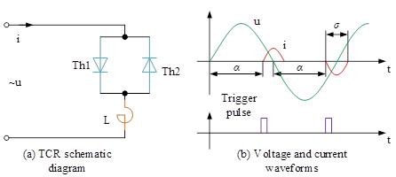
Since the TCR is connected in parallel to the bus, and the voltage distortion on the bus is generally controlled to a small degree. Therefore, it can be assumed that the bus voltage \(v\) is an ideal sinusoidal waveform. and \(\alpha\) is the electrical angle at which the SCR valve starts to obtain a positive voltage drop until it is triggered. known as the triggering delay angle. and \(\sigma\) is that is the time elapsed until the SCR valve is triggered to be in a conduction state. known as the conduction angle. and \(\varpi L\) is the fundamental wave reactance \((\Omega )\) of the reactor. Then there are, \[\label{GrindEQ__23_}\tag{23} i=\frac{\sqrt{2} u}{wL} (\cos \alpha -\cos wt).\]
When \(\omega {\rm t}=180{}^\circ\), \(i\) reaches its maximum value \(i_{\max } =\frac{\sqrt{2} u}{wL} (1+\cos \alpha )\). therefore, the value of reactive power absorbed by the reactor can be controlled by controlling the triggering angle \(\alpha\) of this pair of anti-parallel thyristors.
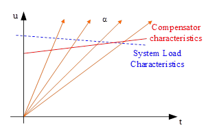
TCR voltage-current characteristics shown in Figure 2, visible TCR voltage-current characteristics is a steady-state characteristic, characteristics of each point is the TCR in the conduction angle for a certain angle is the equivalent susceptibility of the volt-ampere characteristics of a point. the reason why the TCR can be from the voltage-current characteristics of a steady state The reason why the TCR can transfer from one steady state operating point on its voltage-current characteristics to another steady state operating point is the result of the control system constantly adjusting the trigger delay angle, thus constantly adjusting the conduction angle. Obviously, the slope of the characteristic and the intercept on the voltage axis (that is, the normal operating voltage without compensation) are determined by the control system parameters.
TCR basic three-phase wiring
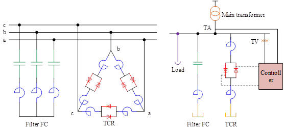
Figure 3 for the TCR + FC-type SVC typical wiring diagram, TCR three-phase wiring form most of the triangular connection, because this wiring form than other forms of line current in the harmonic content is smaller. Individual TCR can only absorb inductive reactive power, so it is often used in conjunction with shunt capacitors (TCR + FC type). In addition, the project is often divided into two parts of each phase of the reactor, respectively, connected to the two ends of the thyristor pair, which allows the thyristor in the reactor damage can be additional protection to prevent when the reactor ends of the short-circuit occurs when the entire AC voltage added to the thyristor valve and lead to its damage.
Basic Composition of Control System
The control system of the TCR generally consists of three components, the detection circuit, which detects the system variables and compensator variables required for control. Control circuit, in order to obtain the required steady-state and dynamic characteristics of the detection signal and the given input processing. Trigger circuit, according to the control signal output from the control circuit to generate the corresponding trigger delay angle of the thyristor trigger pulse. Generally divided into open-loop control and closed-loop control, of which the open-loop control has the advantage of fast response speed and is suitable for load compensation occasions, especially in reducing voltage flicker. Closed-loop control has the advantage of being precise, for transmission compensation, especially which are far away from the load and the power source of the middle point of the transmission line.
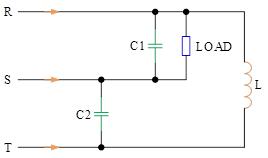
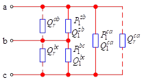
Compensation of three-phase unbalanced loads is shown in Figure 4. Assuming that the supply voltages are balanced, the loads are represented by the triangularly connected network in Figure 4, where \(Y_{1}^{ab}\), \(Y_{1}^{bc}\) and \(Y_{1}^{cc}\) are complex and unequal. Any ungrounded star-connected load can be represented as a triangularly connected form of Fig. by \(Y-\Delta\) transformation.
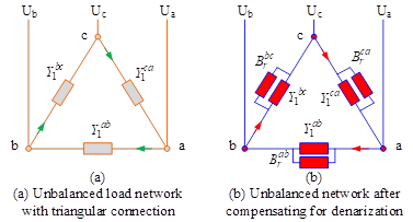
Set, \[\label{GrindEQ__24_}\tag{24} \left. \begin{array}{l} {Y_{1}^{ab} =G_{1}^{ab} +jB_{1}^{ab} } \\ {Y_{1}^{bc} =G_{1}^{bc} +jB_{1}^{bc} } \\ {Y_{1}^{ca} =G_{1}^{ca} +jB_{1}^{ca} } \end{array}\right\}\] Consider first the corrected power factor by connecting in parallel to each load conductor a compensating conductor equal to the negative value of the load conductor so that the load conductor becomes a pure conductor, i.e., let \(B_{r}^{ab} =-B_{1}^{ab}\), \(B_{r}^{bc} =-B_{1}^{bc}\), \(B_{r}^{ca} =-B_{1}^{ca}\), so that all three phases have a power factor of 1 but are still balanced. The phases are pure conductance \(G_{1}^{ab} ,G_{1}^{bc}\) and \(G_{1}^{ca}\). As shown in the figure, in order to balance \(G_{1}^{ab}\), a capacitive conductor \(B_{r}^{bc} =G_{1}^{ab} /\sqrt{3}\) is connected between phases \({\rm b}\) and \({\rm c}\), while an inductive conductor \(B_{r}^{ca} =G_{1}^{ab} /\sqrt{3}\) is connected between phases \({\rm c}\) and a.
Similarly, the pure conductance \(G_{1}^{bc}\) and \(G_{1}^{ca}\) between phases \(b\) and \(c\) can be balanced sequentially in the same way. Combined with the power factor of the corrective electro-nerve, the figure of the triangle in each circuit has three parallel compensations electro-nerve, these electro-nerve added together, you get the three-phase triangular connection of the ideal compensation network: \[\begin{equation}\label{GrindEQ__25_}\tag{25} \left. \begin{array}{l} {B_{1}^{ab} ={-B_{1}^{ab} +\left(G_{1}^{ca} -G_{1}^{bc} \right)\mathord{\left/ {\vphantom {-B_{1}^{ab} +\left(G_{1}^{ca} -G_{1}^{bc} \right) \sqrt{3} }} \right. } \sqrt{3} } } \\ {B_{1}^{bc} ={-B_{1}^{bc} +\left(G_{1}^{ab} -G_{1}^{ca} \right)\mathord{\left/ {\vphantom {-B_{1}^{bc} +\left(G_{1}^{ab} -G_{1}^{ca} \right) \sqrt{3} }} \right. } \sqrt{3} } } \\ {B_{1}^{ca} ={-B_{1}^{ca} +\left(G_{1}^{bc} -G_{1}^{ab} \right)\mathord{\left/ {\vphantom {-B_{1}^{ca} +\left(G_{1}^{bc} -G_{1}^{ab} \right) \sqrt{3} }} \right. } \sqrt{3} } } \end{array}\right\}\end{equation}\]
Thus an ideal compensation network associated with a load can change any unbalanced three-phase load into a balanced three-phase active load without changing the active power exchange between the source and the load.
Since the load conductance is not as easy to measure as the line current and voltage, it is difficult to find the compensator’s conductance. In the following, the symmetrical component method will be used to derive the formula for the compensator conductance expressed in terms of line current and voltage.
Let the unbalanced load in Figure 5 be supplied by the balanced three-phase positive sequence voltage, and the rms value of the neutral voltage of each phase is: \[\label{GrindEQ__26_}\tag{26} \begin{array}{l} {\dot{U}_{a} =\dot{U}} \\ {\dot{U}_{b} =a^{2} \dot{U}} \\ {\dot{U}_{c} =a\dot{U}} \end{array}\] where, \(a=e^{120{}^\circ } =-\frac{1}{2} +j\frac{\sqrt{3} }{2}\) solved by the symmetric component method, the derivation leads to the compensating electro-nerve equation expressed in terms of load current vectors, \[ \begin{equation}\label{GrindEQ__27_}\tag{27} \left. \begin{array}{l} {B_{r}^{ab} ={-\left(Im\dot{I}_{a(1)} +Ima\dot{I}_{b(1)} -Ima^{2} \dot{I}_{c(1)} \right)\mathord{\left/ {\vphantom {-\left(Im\dot{I}_{a(1)} +Ima\dot{I}_{b(1)} -Ima^{2} \dot{I}_{c(1)} \right) 3U}} \right. } 3U} } \\ {B_{r}^{bc} ={-\left(Ima\dot{I}_{b(1)} +Ima^{2} \dot{I}_{c(1)} -Ima\dot{I}_{a(1)} \right)\mathord{\left/ {\vphantom {-\left(Ima\dot{I}_{b(1)} +Ima^{2} \dot{I}_{c(1)} -Ima\dot{I}_{a(1)} \right) 3U}} \right. } 3U} } \\ {B_{r}^{ca} ={-\left(Ima^{2} \dot{I}_{c(1)} +Im\dot{I}_{a(1)} -Ima\dot{I}_{b(1)} \right)\mathord{\left/ {\vphantom {-\left(Ima^{2} \dot{I}_{c(1)} +Im\dot{I}_{a(1)} -Ima\dot{I}_{b(1)} \right) 3U}} \right. } 3U} } \end{array}\right\} \end{equation} \]
In fact, the load is commonly used active power and reactive power to express the reactive power compensation of single-phase load power supply as shown in Figure 5, assuming that its active power is \(P\), reactive power is \(Q_{0}\) according to Steinmetz three-phase balancing calculation method can be balanced by the single-phase load caused by the voltage imbalance, so it can be obtained that the reactive power to be compensated between the phases is as follows: \[\begin{equation}\label{GrindEQ__28_}\tag{28} Q_{C1} =Q\; \; Q_{C2} ={P\mathord{\left/ {\vphantom {P \sqrt{3} }} \right.} \sqrt{3} } \; \; Q_{L} ={P\mathord{\left/ {\vphantom {P \sqrt{3} }} \right. } \sqrt{3} }.\end{equation}\]
The reactive power compensation for supplying three-phase loads is shown in Figure 6, for a three-phase load, assuming that the three-phase load is expressed in terms of active and reactive power as \(P_{l}^{ab} +jQ_{1}^{ab}\), \(P_{l}^{bc} +jQ_{l}^{bc}\), \(P_{1}^{ca} +jQ_{1}^{ca}\).
Then it follows from Steinmetz’s principle, \[\label{GrindEQ__29_}\tag{29} \left. \begin{array}{l} {Q_{r}^{ab} =-Q_{l}^{ab} +{\left(P_{l}^{ca} -P_{l}^{bc} \right)\mathord{\left/ {\vphantom {\left(P_{l}^{ca} -P_{l}^{bc} \right) \sqrt{3} }} \right. } \sqrt{3} } } \\ {Q_{r}^{bc} =-Q_{l}^{bc} +{\left(P_{l}^{ab} -P_{l}^{ca} \right)\mathord{\left/ {\vphantom {\left(P_{l}^{ab} -P_{l}^{ca} \right) \sqrt{3} }} \right. } \sqrt{3} } } \\ {Q_{r}^{ca} =-Q_{l}^{ca} +{\left(P_{l}^{bc} -P_{l}^{ab} \right)\mathord{\left/ {\vphantom {\left(P_{l}^{bc} -P_{l}^{ab} \right) \sqrt{3} }} \right. } \sqrt{3} } } \end{array}\right\}\]
Calculate the capacity to be compensated for each phase according to Eq. 21 . Where the negative sign in front of P indicates inductive reactive power and the positive sign indicates capacitive reactive power. In the actual project, the appropriate compensation capacity is calculated and selected according to the specific conditions of the load.
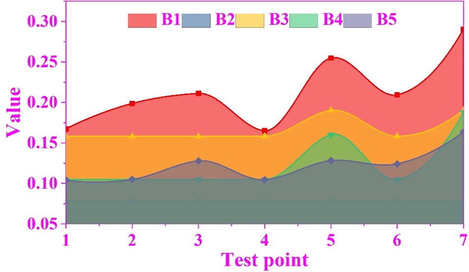
The data of power quality indicators at the test points are shown in Figure 7, and the data of each indicator in this paper were obtained from the 24-hour power quality measurements of switches of 110 kV voltage level under seven substation buildings in area Y by the PW3198 power quality monitoring instrument, and the sampling interval was set to 30 seconds. The selected assessment indicators contain five indicators including voltage deviation and frequency deviation, which are noted as \(B=\left(B_{1} ,B_{2} ,B_{3} ,B_{4} ,B_{5} \right)\), and the values of all five indicators fluctuate steadily in the range of 0 to 9.

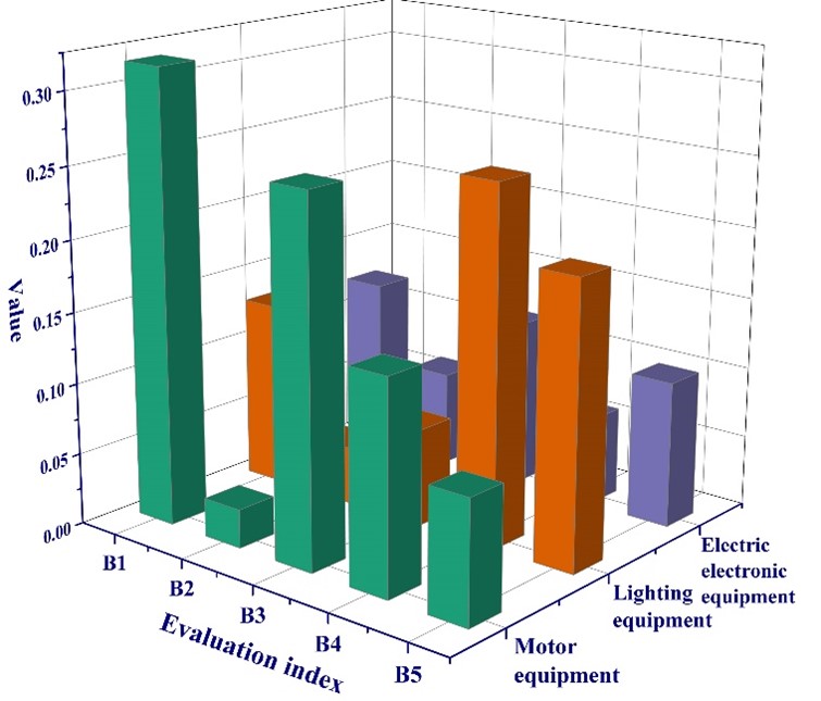
The subjective weights of the assessment indicators of each equipment are shown in Figure 8, because the power quality indicators have different quantitative outlines, and the indicators selected in this paper are all cost-based indicators, so the seven assessment points monitored are mainly to supply power to industrial production, therefore, the respective percentage G of each typical equipment in the industrial electricity load can be calculated: motor equipment G=0.83825, lighting equipment G=0.03515, power electronic equipment G = 0.12611, and then through the review of relevant literature and combined with the equipment attributes of the three equipment under the indicators were assigned, motor equipment assessment indicators in the voltage deviation and frequency deviation weight is larger, lighting equipment in the flicker indicator weight is the largest, the power electronic equipment in the harmonic-related indicators weight is larger, which is consistent with the attributes of each device, so through the classification of the equipment for subjective assignment compared to traditional Therefore, subjective assignment through equipment classification is more reasonable than traditional subjective assignment. Voltage deviation and frequency deviation in the evaluation index of motor equipment have larger weights, flicker index in lighting equipment has the largest weight, and harmonic-related index in power electronic equipment has larger weights, which is consistent with the attributes of each equipment, so subjective assignment through equipment classification is more reasonable than traditional subjective assignment.
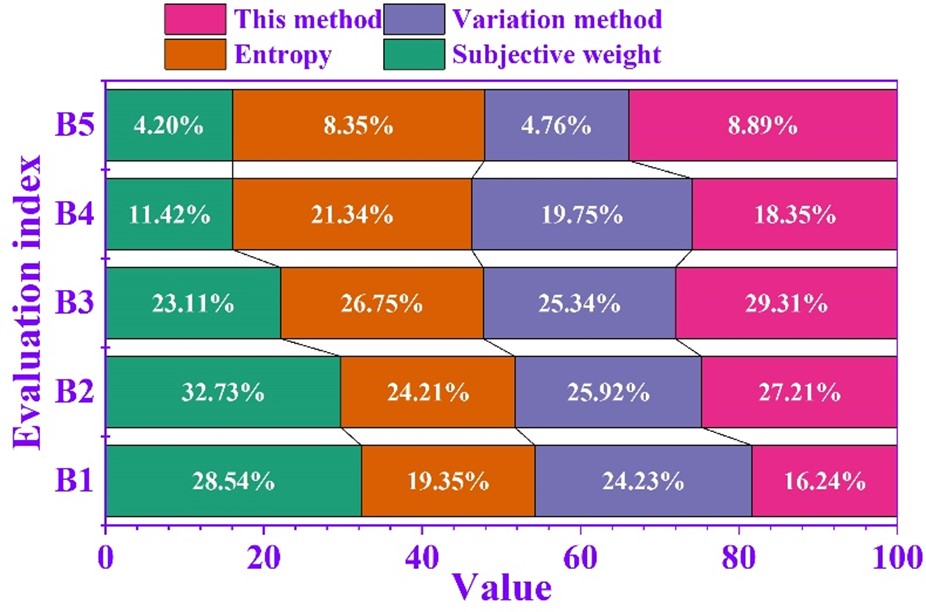
Considering that the adoption of a single subjective weight or objective weight as the final weight of the power quality assessment index is too one-sided, in order to fully synthesize the impact of subjective and objective weights on the results of the assessment of power quality, the weights of the indexes obtained by the different methods are shown in Figure 9, and the differences in the objective weights obtained by using entropy weighting and the coefficient of variation method are relatively small, whereas the gap is larger than that with the subjective weights, and the evaluation method of this paper (8.89% to 29.31%) makes up for the shortcomings of using a single weight that is too one-sided.
However, considering that some indicators may exceed the standard in the actual situation, if the indicator is given a smaller weight, the role of the indicator in the assessment process will be reduced, which will lead to inaccurate assessment results, and the phenomenon that the assessment results do not match with the actual power quality, so this paper adopts the “variable weighting idea” to dynamically adjust the weights of the various assessment indicators of power quality. Therefore, this paper dynamically adjusts the weights of the power quality assessment indicators through the “variable weight idea”. The penalty factor is a=0.1, and the negative factor is b=[7 2 0.2 1 2 1.6 1.6 1.6 1.6 1.6], then the corresponding weight value of each index is adjusted by the variable weight, and the corresponding weight of each index after the variable weight is adjusted is shown in Figure 10. After variable weighting improvement weights were 0.2106, 0.2532, 0.2082, 0.2865.
The combination weight of the flash change of test point 5 and test point 7 was 0.1024, and after variable weighting improvement the weights were 0.1583, 0.18735, which can be seen that the weight of the indicator adjusted by variable weighting ideas increased compared with the original combination weight, thus improving the indicator in the electrical energy This increases the influence of the indicator in the process of power quality assessment, which makes the power quality assessment results more in line with the actual situation. However, the voltage deviation values are higher, and the power quality of pilot 3 and test point 6 is even worse than that of test point 2 in terms of the single assessment index, so the assessment results are obviously not in line with the actual situation, while the adjustment through variable weighting reasonably enlarges the weight of voltage deviation, and the assessment results obtained are more in line with the actual situation of the power quality, so it is reasonable to adjust the weighting through the idea of variable weighting. And the assessment results are basically consistent with the other two methods, so the power quality assessment method proposed in this paper is effective.
This study comprehensively and accurately analyzes the power quality and constructs a scientific assessment system of great significance: firstly, it can help the power sector understand the actual quality level of power in a more comprehensive and detailed way, so that it can have an overall grasp of the strengths and weaknesses of the quality of power, discover some existing power quality problems in a timely manner and take corresponding measures to stabilize the power system and guarantee the quality of power, so that it can build the world’s leading energy Internet enterprise with Chinese characteristics as early as possible. The energy Internet enterprise with Chinese characteristics will be built as soon as possible.
Secondly, through the assessment of power quality grading, to realize the market positioning of different levels of power quality, to ensure that power pricing is reasonable, so as to facilitate the users to reasonably purchase power and arrange production, reduce the disputes between supply and demand sides, and at the same time, for some users, especially some of the sensitive users who have special requirements for the power they need, it can help the users to understand the actual situation of the power they use, and apply to the relevant power supply department in time when the power they use fails to satisfy their needs. At the same time, for some users, especially some sensitive users with special requirements, it can help them understand the actual situation of the power used, and apply for modification to the relevant power supply department in time when the power used cannot meet their needs. Moreover, from the perspective of development, the development of society must be accompanied by a large number of equipment replacement, which means that the continuous development and reform of the power grid will always be accompanied by power quality problems, so the comprehensive assessment of power quality will continue to have new requirements with the advancement of the times to join.
The simulation parameters are shown in Table [t3]. In order to verify the correctness and feasibility of the proposed topology and the differential beat-less-repeat control strategy, the simulation model is constructed on Matlab 2016 simulation software with reference to the circuit structure in Fig. 3.1. In the simulation The active power of the building is 2.5 MW and the reactive power is 2 MVar; The active power of building \(\beta\) is 7MW and the reactive power is 5.8MVar. 3rd, 5th, 7th\(\mathrm{\cdots }\)19th harmonic current sources are used to simulate the harmonics generated in each building. The number of TSC configurations is two, the first one has a capacity of 1.8MVar, the second one has a capacity of 3.6MVar and the capacity of the 3rd and the 5th filtering branches are equal in each group of SVCs.
| Parameter | Numerical value | Parameter | Numerical value |
|---|---|---|---|
| Three-phase grid short circuit capacity | 1000MVA | Dc capacitance | 0.1\(\Omega\) |
| Three grid voltage | 110Kv | Direct current voltage reference | 50mF |
| Master variable rated capacity | 30MVA | Dc PI | 20000V |
| Primary variable three-phase transformer | 27.5kV | Direct current voltage initial value | P=0.8,I=5 |
| Filter inductance | 10.5 kV | Carrier frequency | 19500V |
| Equivalent resistance | 2mH | Dc capacitance | 10kHz |
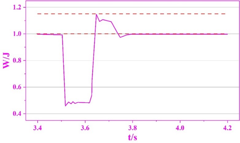
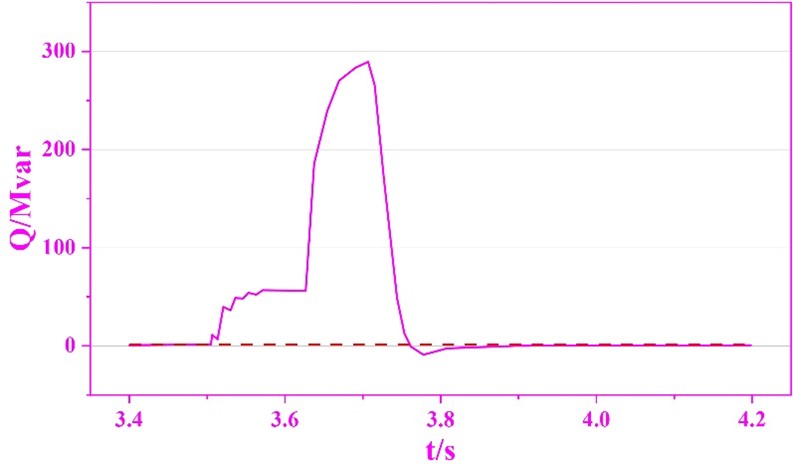
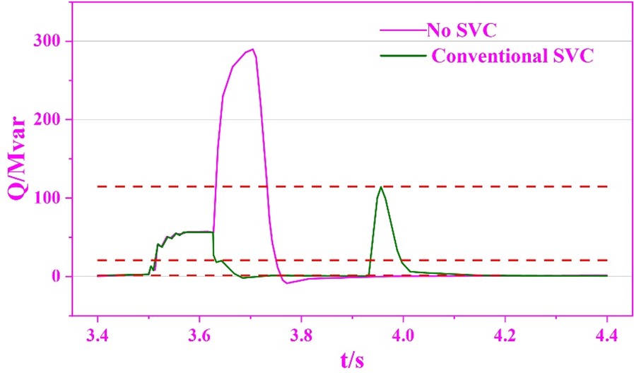
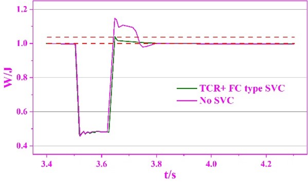
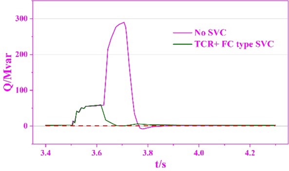
Simulation settings: set the fault generating element to generate a three-phase grounded short-circuit fault, and set the fault occurrence time and duration of the fault timing control logic element to 3.5s and 0.12s, respectively, and the simulation result waveforms when there is no SVC power quality control are shown in Figure 11, in which (a) and (b) are the target 230kV bus power and SVC no power output, respectively. As can be seen from the figure, after a three-phase grounded short-circuit fault occurs in the system at the moment of 3.5s, the target 230kV bus power W falls rapidly to 0.45457J, at this time, even if the SVC releases all the capacitive reactive power, but due to the voltage is too low, the reactive power support provided is very limited, i.e., only 56.6 Mvar, and it can only raise the W to 0.4822pu. At the moment of 3.62s, the fault is cleared and the power recovers rapidly. After the fault is cleared in 3.62s, the power is restored quickly, and the lag in the response of SVC to the transient power makes the capacitive reactive power output from SVC suddenly increase to 295Mvar in a short time, which leads to the increase of W to 1.1511J, which is larger than the threshold value of the bus bar for the protection of the power of 1.15J. Thus, it can be seen that the main reason for the overshooting of the power after the fault lies in the SVC.
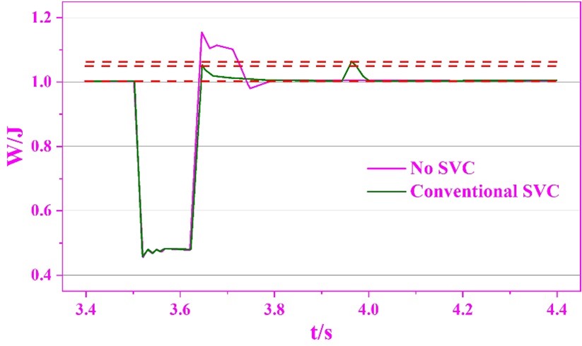
The simulation results of applying the conventional blocking power quality control strategy under the same working condition are shown in Figure 12, where (a) and (b) are the target 230kV bus power and SVC reactive power output, respectively. The conventional blocking LV protection control strategy balances the inductive reactive power output from the TCR with the capacitive reactive power output from the capacitive equipment to make the SVC output zero, which can inhibit the reactive power surge after the fault is cleared and avoid the resulting voltage overshoot, corresponding to the surge value of reactive power reduced from 295 Mvar to 23 Mvar and the overshoot value of power reduced from 1.1511 J to 1.0505 J. However, when the SVC is released from blocking, the SVC output will be reduced from 295 to 23 Mvar. However, when unlocking the SVC, the output of the main PI regulator is not equal to the pre-fault value, and the SVC can not be controlled immediately because of the response lag, resulting in large fluctuations in the output of the SVC and the electric energy J: the output of the SVC is first rapidly increased to 114.55 Mvar and the electric energy W is raised to 1.054 J, and then it is not until the moment of 4.1s that the SVC output is adjusted to the pre-fault value, i.e., 0.5 Mvar. adjusted to the pre-fault value, i.e., 0 Mvar, and stabilized the electrical energy at the target value of 1.0 J.
Applying the new SVC low power quality control strategy proposed in this paper in the same working condition. Summary of the simulation results waveforms are shown in Figure 13, where (a) \(\mathrm{\sim}\) (d) are the bus 230kV bus power, SVC reactive power output, the equivalent electro-nerve reference value, thyristor trigger angle. The results show that at the moment of 3.5s, a three-phase short-circuit fault occurs in the system, resulting in a rapid drop of power J. The main PI regulator quickly changes the output of the Energizer reference value to 0 (adjusting the trigger angle to the limit value of 169.93\(\mathrm{{}^\circ}\)) to control the inductive reactive output of the TCR at least in order to maximize the release of capacitive reactive power from the capacitive equipment to provide reactive power support to the system. After meeting the conditions of 0.6J below the threshold value and 100ms delayed judgment time at 3.607s, the new SVC power quality control starts: after shielding the original input and output of the main PI regulator, input the equivalent voltage deviation e, i.e., 0.004639pu, calculated from the pre-failure Bref1, i.e., 0.05374S, and at the same time input the locked trigger angle, i.e., 114.87\(\mathrm{{}^\circ}\), to the TCR trigger control link. \(\mathrm{{}^\circ}\) is input to the TCR trigger control link to prepare the pulse signal and exit the TSC. At the moment of 3.62s when the fault clearing voltage starts to recover rapidly, since the TCR has been controlled to output inductive reactive power according to the trigger angle, it can:
offset with the capacitive reactive power that surges at this time, suppressing the reactive power surge and voltage overshoot: there is no reactive power surge after the fault is cleared and the electrical energy reaches only 1.0435 J at the maximum.
Reducing the magnitude of the post-fault power change helps the system to recover to the pre-fault state faster and more stably, and reduces the impact of the transient process on the system caused by the fault: W first rises to 1.1365 J due to the reactive power surge during the SVC fixed power control, and then falls to 0.9654 J due to the large amount of inductive reactive power output from the TCR. However, during the new low power quality control process, the reactive power is always locked to the pre-fault trigger angle due to the fact that it has been locked to the pre-fault trigger angle , so the power can be gently reduced from the highest 1.0435 J to the target value of 1.0 J. After the conditions of greater than the threshold value of 0.7 J and a delay of 300 ms are satisfied at the moment of 3.931s, the novel SVC low power quality control is turned off. Since the output of the main PI regulator increases continuously from 0 according to the equivalent deviation e after the novel low power quality control is activated (but does not control the SVC) and is equal to the pre-fault value when the low power quality control is turned off, the output of the SVC is maintained unchanged during the restoration of the fixed power main control, which ensures the stabilization of the building’s electrical energy.
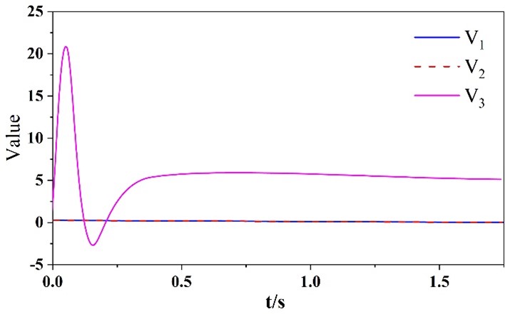
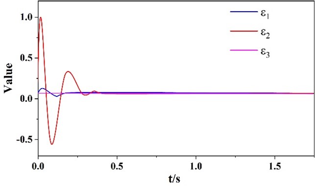
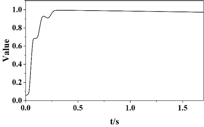
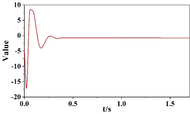
The simulation results of the closed-loop signals are shown in Figure 14 and Figure 14. From Figure 11 and Figure 12, it can be seen that the compensated tracking error \(v_{i} \left(i=1,2,3\right)\) and the error compensation variable \(\varepsilon _{i} \left(i=1,2,3\right)\) possess boundedness. Figure 13 and Figure 14 show the variation curves of the control input signal for the adaptive rate and SVC controllers, respectively. From the simulation results, it can be seen that the control scheme proposed in this chapter ensures that the closed-loop signal enters the bounded region in a limited time. In recent years, as the complexity and size of building power supply systems increase, the problem of operational stability has become increasingly prominent. The loss of stability of the power supply system can cause great losses and damages to the whole building. In this subsection, the stability control problem of a single machine infinity power system with SVC is investigated, and a new finite time fuzzy adaptive controller is designed considering the existence of unknown nonlinear dynamics and external disturbance signals in the system. The proposed control strategy realizes the stabilization control of all state variables in finite time, thus ensuring the voltage stability at the access point of SVC equipment. Different from the previous finite-time control scheme a novel finite-time filter is introduced and the error compensation variables are designed to ensure that the derivatives of the virtual control signal can complete the approximation in finite time. Finally, the effectiveness of the proposed control scheme is proved by both theoretical and experimental means. As an emerging reactive power compensation technology, the static reactive power compensator can efficiently balance the reactive power of the power supply system, effectively reduce the power loss, improve the stability of the power supply to the building, and to a certain extent, effectively control the system’s low-frequency vibration.
Improvement of power quality is a hot issue in the future social development, but also the key direction of the future development of power grid technology. The research and design of reactive power compensation device is an essential part of this, and the design of a cost-effective reactive power compensation device will have its broad application prospects. Although the low-voltage TCR + TSC-type SVC designed in this paper can meet the requirements of practical applications, and has a certain degree of technical sophistication, but in the following aspects there are still some defects to be improved in the future action:
Although the design of reactive power compensation device in this paper takes into account the system of anti-interference hardware circuit design, but for the reactive power compensation device grid-connected work in the process of harmonic generation, the electromagnetic interference of the working environment as well as reasonable anti-interference hardware circuit design has to be followed by further systematic research in order to improve the stability and reliability of the device operation.
In the low-voltage grid compensation reactive power control, with the continuous updating and improvement of modern control theory, the precise calculation and control of compensation reactive power, the compensation of the device’s dynamic response is more rapid and stable will also be a worthy of in-depth research in the future.
This study comprehensively analyzes the assessment and control of building power quality, collects and analyzes data through online monitoring technology, and establishes a complete system of power quality technical indicators. In terms of power quality assessment, the scientific quantitative assessment of building power quality is realized through the methods of standardized processing and weight determination. The test results show that the power quality index fluctuates within the range of 0 to 9, effectively reflecting the actual power quality status and proving the effectiveness of the assessment system.
In terms of power quality control, the focus is on analyzing the static reactive power compensation device (SVC) and its application effect in power quality control. Through an in-depth analysis of the working principle and control strategy of SVC, and combined with practical simulation experiments, this study demonstrates the important role of SVC in enhancing power quality and stabilizing grid operation. The results of simulation experiments show that SVC can effectively control power quality and mitigate the impact of grid faults on power stability, thus enhancing the overall performance of the power system.
This study not only constructs a comprehensive building power quality assessment system, but also demonstrates the possibility and effectiveness of improving power quality through the application of practical control techniques. This is of great significance for the stable operation of the power system and the improvement of power quality, which not only helps the power sector to understand the actual quality level of power more comprehensively and carefully, and to find and solve power quality problems in time, but also provides a scientific basis for power pricing and consumer demand for power.
This research was supported by one of the phased results of the 2021 Guangxi University Young and Middle-aged Teachers’ Scientific Research Basic Ability Improvement Program: Research on Civil Building Power Quality Detection and Governance (Program Number: 2021KY1077).