People’s consumption concept and consumption mode with the continuous growth of social and economic growth, e-commerce logistics enterprises such as spring, the people’s consumption is no longer limited to brick-and-mortar stores, which gives rise to the problem of who to distribute, how to distribute, distribution speed, distribution costs [1, 2]. Therefore, the current e-commerce logistics enterprises put forward new issues, based on the social contradictions of the new era, in the logistics openness, technology level, innovation capacity, etc. should take effective countermeasures in order to optimize the logistics and distribution paths, in the fierce competition to convert the traditional logistics and distribution model, improve the quality of distribution services and efficiency, and bring a good experience for the user, so that the distribution of logistics enterprises in the tide of the market economy to stand firm, to achieve sustainable development [3, 4].
The rapid change of information technology, prompting the rapid rise of e-commerce, and led to the rapid development of the logistics industry, but at the same time logistics and distribution has also become a key factor restricting the development of e-commerce, so optimize the distribution routes, reduce logistics costs, improve customer satisfaction is to improve the competitiveness of the enterprise key [5, 6]. E-commerce from the technical level to solve the information flow, business flow, capital flow of the transmission of space and transmission time, and really affect or prevent its development of the key factors focused on the logistics of this problem [7, 8]. At this stage, the major e-commerce enterprises online promotions, offline promotion of the competitive situation is intense, from the explosive rise of e-commerce enterprises, poorly run e-commerce enterprises have to shut down, merger, until today’s Ali, Jingdong, Dangdang and other large-scale e-commerce enterprises, such as multi-purpose tripod [9, 10]. As an important factor in the realization of e-commerce – logistics and distribution, has become an important fulcrum in the process of e-commerce, logistics problems have also become a bottleneck in the development of e-commerce [11, 12]. Especially for the distribution of fresh and perishable food, the primary goal is to complete the distribution task in as short a time as possible [13, 14]. Through the use of artificial intelligence algorithms – ACO algorithms to optimize the distribution, can effectively solve the e-commerce logistics and distribution in the path optimization problem [15, 16].
Considering the limitations of traditional methods in dealing with complex logistics networks, we chose the ant colony algorithm as the main research tool, which starts with a detailed analysis of the e-commerce logistics system, and clarifies the optimization objectives and constraints, and then we construct an ant colony algorithm model adapted to e-commerce distribution characteristics, and through algorithmic adjustments and parameter optimization, we can effectively deal with e-commerce logistics path optimization problems. We verify the effectiveness and practicality of the algorithm through simulation experiments on test cases of different sizes and complexities, and the whole research process focuses on improving the performance of the algorithm, aiming at realizing shorter delivery paths and lower transportation costs.
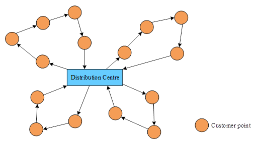
Distribution path optimization problem schematic shown in Figure 1. distribution path optimization problem refers to certain constraints based on the planning of vehicles from the distribution center to the customer’s transport route, in order to maximize the profit of the enterprise. specifically, there is a set of customer demand points, each demand point exists in different demand, distribution centers have a group of transport vehicles to provide distribution services, from the distribution center, distribution vehicles will be in accordance with the path of the pre-planned for the customer to carry out logistics and distribution of the point in a certain number of constraints limitations on the driving route to carry out the design of a more reasonable plan, to achieve the shortest distance to travel, the lowest distribution into the optimal goal.
The distribution path problem components are as follows;
Distribution center
Vehicles in the distribution center to load the goods required by the customer, and in the end of the distribution service back to the distribution center. in a logistics distribution system, there may be a (single-stage distribution center) or several (multi-level distribution center) distribution center.
Service demand point
Service demand points include a variety of warehouses, retail stores, etc. Customers need the number of deliveries and pickups, access time constraints, etc. constitutes the constraints of the path problem.
Delivery vehicles
Vehicles are the means of transportation required to provide pickup and delivery services to various customer nodes. the main elements include the type of vehicle, fixed cost, transportation cost, maximum distance traveled, and maximum loading capacity.
Transportation of goods
The goods to be transported are items purchased or sent by the customer, and the main elements to be considered include the weight of the goods, packaging, the type of goods, and the time of delivery or transportation of the goods, etc. The main elements to be considered include the weight of the goods, packaging, the type of goods, and the time of delivery or transportation of the goods.
Transportation network
Transportation network is a network consisting of nodes (i.e., distribution centers, customers, parking lots, etc.), undirected edges and directed maps.
Constraints
In order to realize the problem of distribution route optimization in practical applications, it is necessary to add some conditions to limit the main constraints, including the customer’s requirements on the arrival time of the goods, the actual number of vehicles loaded with the limitations, the location of the distribution center, and so on.
Optimization objective
The optimization objective of the distribution route problem can be divided into single objective and multi-objective problems according to the number of more common objective functions include the minimum number of transport vehicles, the total distribution distance is the shortest, the total transport time is the shortest, the total cost is the lowest and so on.
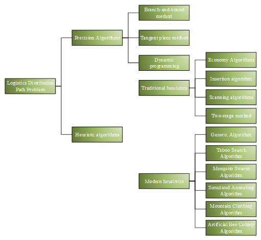
Path optimization problem solving specific algorithm classification shown in Figure 2. usually solving the e-commerce logistics distribution path optimization problem of many algorithms, including accurate algorithms and heuristic algorithms, this paper is mainly seven heuristic algorithms as the entry point to the analysis of the e-commerce logistics distribution path optimization problem, heuristic algorithms are divided into the traditional heuristic algorithms and modern heuristic algorithms, modern heuristic algorithms include genetic algorithms, forbidden search algorithms, ant colony algorithms, simulated annealing algorithms, climbing algorithms.
The annealing algorithm is inspired by the annealing process of solid material, in the annealing algorithm, the initial solution is considered to be a high temperature state, and then by introducing random disturbance in the solution space, and accepts the new solution based on the specific criterion, the algorithm is more suitable for the combination optimization problem and continuous optimization problem. The ant colony algorithm is more advantageous in solving complex problems and global search, and all this method is used as a method of study.
The objective function of the e-commerce logistics distribution model constructed in this paper includes distribution revenue, distribution subsidy and distribution cost, of which distribution cost includes four parts, i.e., distribution and transportation cost, vehicle fixed activation cost, soft time window penalty cost, and cargo damage cost.
Distribution revenue
In the process of e-commerce logistics distribution, the distribution revenue is composed of the revenue of express delivery to each site and the revenue of retrieving products, and the total revenue obtained is proportional to the number of pickups and deliveries: the total revenue obtained is proportional to the number of pickups and deliveries. \[\label{GrindEQ__1_}\tag{1} R=\sum\limits_{i=1}^{n}\sum\limits_{k=1}^{m}\left[r_{1} q_{i} +r_{2} p_{i} \right] y_{ik}.\]
In Eq. 1 , \(r_{l} q_{i}\) denotes the revenue gained from delivery at node i, and \(r_{2} p_{i}\) denotes the revenue gained from pickup at node i.
Distribution subsidies
The city government will provide certain subsidies to the logistics enterprise, the subsidy consists of the distribution of express delivery subsidies, pick-up subsidies and fuel subsidies, so the distribution subsidies for logistics enterprises as shown in Eq. 2 . \[\label{GrindEQ__2_}\tag{2} B=\sum\limits_{i=1}^{n}\sum\limits_{k=1}^{m}\left[r_{3} q_{i} +r_{4} p_{i} \right] y_{ik} +\sum\limits_{i=0}^{n}\sum\limits_{j=0}^{n}\sum\limits_{k=1}^{m}r_{5} d_{ij} x_{ijk}.\]
In Eq. 2 , \(r_{3} q_{i}\) denotes the delivery subsidy at node i, \(r_{4} p_{i}\) denotes the pickup subsidy at node i, and \(r_{5} d_{ij}\) denotes the fuel subsidy from node i to j.
Distribution costs
Distribution vehicles in the transportation process will produce distribution and transportation costs, including depreciation costs and fuel costs incurred in the vehicle distribution process.The total distribution and transportation costs of distribution vehicles \(C_{1}\) as shown in Eq. 3 , \[\label{GrindEQ__3_}\tag{3} C_{1} =\sum\limits_{i=0}^{n}\sum\limits_{j=0}^{n}\sum\limits_{k=1}^{m}c_{1} d_{ij} x_{ijk}.\]
The sum of the salaries paid to the delivery personnel, the cost of insurance and the cost of purchasing the delivery vehicle is counted as the fixed cost of the vehicle.The fixed start-up cost of the delivery vehicle is shown in Eq. 4 , \[\label{GrindEQ__4_}\tag{4} C_{2} =\sum\limits_{j=1}^{n}\sum\limits_{k=1}^{m}c_{2} x_{0jk}.\]
In Eq. 4 \(x_{0jk}\) indicates that all distribution services start from node 0, i.e., from the town distribution center.
In order to reduce the logistics enterprises to save distribution costs appear in the phenomenon of hoarding distribution courier, adding a soft time window penalty cost. \(\left[ET_{i} ,LT_{i} \right]\) is the distribution time range required by the customer i, \(t_{i}\) for the distribution vehicle to reach the customer i time, the distribution vehicle does not necessarily have to be in the customer’s expected to arrive within the time period, in excess of the customer’s specified range of time to reach the customer will still be received, but need to pay the corresponding waiting or late arrival time length in accordance with the early or late arrival time, or the time to pay the corresponding waiting or late arrival time. Late to the length of time to pay the corresponding waiting or late to the penalty fee, the penalty function for the formula 5 shows. \[\label{GrindEQ__5_}\tag{5} P(t)=\left\{\begin{array}{cc} {E_{a} \max \left(\left(ET_{i} -t_{i} \right),0\right)} & {t_{i} \le ET_{i} } \\ {0} & {ET_{i} \le t\le LT_{i} } \\ {L_{a} \max \left(\left(t_{i} -LT_{i} \right),0\right)} & {t_{i} \ge LT_{i} } \end{array}\right.\]
Product upstream problems, the transportation process is too long will cause the deterioration of agricultural products and thus produce the cost of loss, the cost of loss of goods is mainly in the transportation process due to changes in time and the cost.
In this paper, the cargo deterioration function is used to represent the change process of product perishable damage, i.e., \(S(t)=e^{-\alpha t}\), where \(S(t)\) is the existing quality of agricultural products, \(\alpha\) is the cargo deterioration rate of perishable products at a certain temperature, and \(t\) is the transportation time of the product.Assuming that the inside of the compartments in the process of agricultural products recycling is at a constant temperature, and only the length of time of the road transportation is taken into consideration to affect the quality of the cargoes, the change of the temperature has no impact on the cargoes.The total deterioration costs of the transportation process in the case of recycling of agricultural products, \(C_{4}\) is expressed in Eq. 6 as follows, \[\label{GrindEQ__6_}\tag{6} C_{4} =\sum\limits_{i=0}^{n}\sum\limits_{j=0}^{n}\sum\limits_{k=1}^{m}c_{4} p_{i} \left(1-e^{-\alpha t\eta } \right)x_{ijk}.\]
To sum up, the enterprise distribution profit is equal to the sum of distribution revenue and distribution subsidy minus all kinds of costs; therefore, the total optimization objective function is shown in Eq. 7 as follows, \[\label{GrindEQ__7_}\tag{7} \begin{array}{rcl} {F} & {=} & {R+B-C_{1} -C_{2} -C_{3} -C_{4} }. {} \end{array}\]
Decision variable constraints
\[\label{GrindEQ__8_}\tag{8} \begin{array}{l} {x_{ijk} =\left\{\begin{array}{l} {1\; \text{Vehicle}{\rm \; }k{\rm \; }\text{travelling}{\rm \; }\text{from}{\rm \; }i{\rm \; }to{\rm \; }j} \\ {0\; \text{Otherwise}} \end{array}\right. } \\ {y_{ik} =\left\{\begin{array}{l} {1\; \text{Customer}{\rm \; }i{\rm \; }\text{is}{\rm \; }\text{delivered}{\rm \; }\text{by}{\rm \; }\text{vehicle}{\rm \; }k} \\ {0\; \text{Otherwise}} \end{array}\right. } \end{array}\]
In Eq. 8 , \(x_{ijk}\) means that when distribution vehicle \(i\) is directly from logistics node \(j\), it takes the value of 1, otherwise it is 0. \(y_{ik}\) means that when distribution vehicle \(k\) carries out distribution for logistics node \(i\), it takes the value of 1, otherwise it is 0.
Start and end constraints \[\label{GrindEQ__9_}\tag{9} \begin{array}{l} {\sum\limits_{j=0}^{n}x_{0jk} =1\forall k\in K} \\ {\sum\limits_{i=0}^{n}x_{i0k} =1\forall k\in K} \end{array}\]
Eq. 9 indicates that the distribution vehicle k starts distribution from the distribution center, and returns to the distribution center after completing all the rural customer point distribution services, and each distribution vehicle only carries out a path of distribution services.
Path continuity constraint. \[\label{GrindEQ__10_}\tag{10} \sum\limits_{i=0}^{n}x_{ipk} -\sum\limits_{j=0}^{n}x_{pjk} =0\forall p\in N,k\in K.\]
Eq. 10 indicates that the delivery vehicle k makes a delivery for i and then leaves to make a delivery for the next rural customer point.
Uniqueness constraint \[\label{GrindEQ__11_}\tag{11} \sum\limits_{i=0}^{n}\sum\limits_{k=1}^{m}x_{ijk} =1\forall j\in N,i\ne j.\]
Eq. 11 indicates that each customer point is visited only once.
Relational constraints on decision variables. \[\label{GrindEQ__12_}\tag{12} \begin{array}{l} {\sum\limits_{i=0}^{n}x_{ijk} =y_{jk} \forall j\in N,k\in K} \\ {\sum\limits_{j=0}^{n}x_{ijk} =y_{ik} \forall i\in N,k\in K} \end{array}\]
Eq. 12 indicates that each customer point has a path connection between them.
Vehicle loading capacity related constraints \[\label{GrindEQ__13_}\tag{13} \sum\limits_{i=l}^{n}Q_{0jk} =\sum\limits_{i=l}^{n}\sum\limits_{j=I}^{n}q_{i} x_{ijk} \le Q\forall k\in K.\]
Eq. 13 indicates that the loading capacity of distribution vehicle k at the time of departure from the distribution center is equal to the demand at all customer points in the distribution process, and that this initial loading capacity does not exceed the maximum loading capacity. \[\label{GrindEQ__14_}\tag{14} \sum\limits_{i=1}^{n}Q_{i0k} =\sum\limits_{i=1}^{n}\sum\limits_{j=1}^{n}p_{i} x_{ijk} \le Q\forall k\in K.\]
Eq. 14 indicates that distribution vehicle k returns to the distribution center with a load equal to the number of pickups at all rural customer locations along the distribution path, and returns with a vehicle load that does not exceed the maximum loading capacity. \[\label{GrindEQ__15_}\tag{15} 0\le Q_{ijk} \le Q\forall i,j\in N,k\in K.\]
Eq. 15 indicates that the loading capacity of distribution vehicle k at any point in the distribution process is non-negative and does not exceed the maximum loading capacity:. \[\label{GrindEQ__16_}\tag{16} \sum\limits_{i=1}^{n}\sum\limits_{k=1}^{m}Q_{ipk} +\sum\limits_{i=1}^{n}\sum\limits_{k=1}^{m}\left(p_{p} -q_{p} \right) x_{ipk} =\sum\limits_{i=1}^{n}\sum\limits_{k=1}^{m}Q_{pjk} \forall p\in N,k\in K\]
Eq. 16 represents the load balancing constraint of distribution vehicle k before and after logistics node p.
The colony algorithm simply means that when one ant finds food, more and more ants will reach the same place, resulting in more and more pheromone buildup on that path, attracting more ants to come, while other paths that do not find food are ignored. the path with the highest concentration of pheromone is the best foraging path.
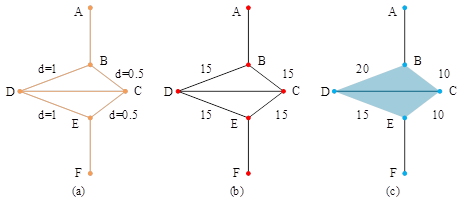
The simulation diagram of the ant colony algorithm is shown in Figure 3, the two main factors affecting the solution are pheromone and environment. A represents the ant’s colony, F represents the food, CD represents the obstacles encountered from the ant’s colony to the food, and the various line segments between A and F represent different foraging paths from the ant’s colony A to the food F. Depending on the length of the paths, different weights are assigned to each path, and it is very obvious from the figure that the shortest path is A-\(\mathrm{>}\)B-\(\mathrm{>}\)C-\(\mathrm{>}\)E-\(\mathrm{>}\)F., we assume that the probability of ants passing through each path is the same, that is to say, the number of ants passing through the two paths of BDE and BCE is the same, then it is obvious that the paths of BDE are longer than the paths of BCE, which leads to the number of repeated passages of ants on BCE is more than that of BDE within the same period of time, which triggers more ants to participate in the path, so the cycle forms a positive feedback, and finally the shortest path shown in Figure 3 is formed.
Synergistic mechanism, each ant will leave pheromone when it traverses the path it has traveled, and at the same time, it will perceive the path pheromone in the process of walking, and the pheromone is the carrier of information exchange in the process of ants’ walking.
Selection mechanism, when the ants perceive pheromone during walking, the higher the pheromone concentration of the current path, then the ants will choose the path with high pheromone concentration with high probability, that is, the path selection is proportional to the pheromone concentration.
Update mechanism, as long as the ants choose the shorter path, then the same time the path through the number of ants will be more, so that the pheromone concentration left on this path is higher, so the formation of positive feedback, the final pheromone concentration of the highest path is the shortest path.
According to the above analysis, the working mechanism of a group of algorithms can be summarized as follows;
Let there be \(m\) only ants, \(d_{ij}\) denotes the distance that ants walk from \(i\) to \(j\), the pheromone concentration of ants during the whole walking process from \(i\) to \(j\) is \(\tau _{{\rm ij}}\), and the heuristic function is \(\eta _{j} =1/d_{ij}\), then according to the algorithm’s transfer rule, that is, the probability distribution of ants exactly choosing that path, at the very beginning, since the pheromone distribution of each path is completely consistent, assuming that the concentration is C (constant), then there is \(\tau _{ij} =C\), remember the ants in the \(t\) moment when a consistent ant \(k\) from \(i\) to \(j\) the probability of transfer occurs as \(P_{ij}^{k}\), then there is the following formula 17 probability of transfer formula, \[\label{GrindEQ__17_}\tag{17} P_{ij}^{k} =\left\{\begin{array}{lll} {\frac{\tau _{ij}^{\alpha } (t)\eta _{\bar{j}}^{\beta } (t)}{\sum\limits_{s\in\text{allowed}_{i} }\tau _{ij}^{\alpha } (t)\eta _{\bar{j}}^{\beta } (t)} } & {if} & {s\in \text{allowed}_{k} } \\ {0} & {} & {\text{otherwise}} \end{array}\right.\]
In Eq. 17 , \(allowed\left(k=1,2,\cdots ,n-1\right)\) represents the ant \(k\) in the next path node selection, that is, the set of all the remaining nodes to be visited, \(\alpha =\) information heuristic factor, \(\beta =\) expectation heuristic factor. as the ants search iteration, the path pheromone concentration of the path increases, it is very likely to override the initial heuristic information for the ants path selection, so it is necessary to update the path of the path of the pheromone processing, the ants every time to complete traversal of the path, the path of the pheromone update is computed as follows as shown in Eqs. 18 and 19 . \[\label{GrindEQ__18_}\tag{18} \tau _{ij} (t+1)=\rho \tau _{ij} (t)+\tau _{ij} (t,t+1),\] \[\label{GrindEQ__19_}\tag{19} \Delta \tau _{ij} (t,t+1)=\sum\limits_{k=1}^{m}\Delta \tau _{ij}^{k} (t,t+1).\]
In the above equation, \(\rho\) represents the volatility coefficient of pheromone, \(0<\rho <1\), and the corresponding \(\left(1-\rho \right)\) represents the attenuation of information, i.e., the loss of pheromone on the path \(j\), \(\Delta \tau _{ij}^{k}\) represents the amount of pheromone left behind by the ants \(k\) after traversing the path \(ij\) for one time, and \(\Delta \tau _{ij}\) represents the pheromone total of all ants after traversing the path \(ij\) for one time, which means the pheromone increment of all the ants on the path \(ij\).
According to the different updating mechanisms, the corresponding pheromone updating models can be subdivided into the following models;
Ant perimeter model, the corresponding formula is as follows, \[\label{GrindEQ__20_}\tag{20} \Delta \tau _{1j}^{k} =\left\{\begin{array}{ll} {\frac{Q}{L_{k} } } & {\text{if}} \\ {0} & {\text{otherwise}} \end{array}{\rm }\right.\]
This model is a global update model, that is, as long as the ant completes a full search from i to j, then the pheromone on the path is updated once. \(Q\) in the above equation represents the total amount of pheromone, and \(L^{k}\) denotes the total amount of paths that ant k has passed through after traversing once.
Ant volume model, the corresponding formula is as follows, \[\label{GrindEQ__21_}\tag{21} \Delta \tau _{ij}^{k} =\left\{\begin{array}{cc} {\frac{Q}{d_{1j} } } & {\text{if}} \\ {0} & {\text{otherwise}} \end{array}\text{Ant}{\rm \; }k{\rm \; }\text{passes}{\rm \; }\text{through}{\rm \; }\text{path}{\rm \; }\left(ij\right)\right.\]
This is well explained, that is, the ratio of the total amount of information to the path length as the pheromone increment.
Ant-density model, the corresponding formula is as follows, \[\label{GrindEQ__22_}\tag{22} \Delta \tau _{in}^{k} =\left\{\begin{array}{ll} {Q} & {\text{if}} \\ {0} & {\text{otherwise}} \end{array}{\rm }\right.\]
Similar to the ant measure model, it belongs to a local pheromone updating model.
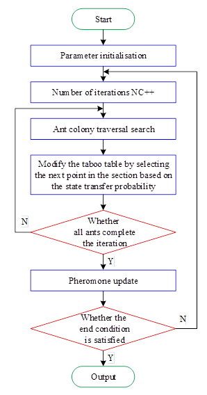
The flow of ACO algorithm is shown in Figure 4, and the specific process steps are described as follows.
The first step is to initialize the parameters of the ant colony algorithm, including the maximum number of iterations Nmax and the node information table of the ants’ paths, which are used to randomly distribute m ants into the node information table.
In the second step, the specific iteration number Nc++ is set during the running process of ACO algorithm, while m ants start the path node search.
In the third step, according to the previously mentioned probability formula 17 , the state transfer of the ants is started, while the pheromone and forbidden node information table on the path ij is updated after every path ij traveled by the ants.
The fourth step is to determine whether the ants have finished searching all the forbidden node information tables, if not, repeat the third step until all the searches are completed, then jump out of the loop to calculate the total distance of the paths traveled by the ants, and obtain the optimal solution of the loop.
In the fifth step, according to the current optimal solution, update the pheromone concentration on each path, and at the same time, set the optimal solution just found out as the current optimal solution.
Step 6, after the completion of the current iteration, determine whether the current number of iterations exceeds the maximum number of iterations, if yes, then directly jump to the next step, if not, then jump to the second step and repeat the execution.
The seventh step, that the number of iterations has reached the maximum number of iterations initially set, then the iteration should be terminated at this time, the ant colony algorithm search is complete, the system outputs the optimal solution for path optimization.
Stochastic rules
In this paper, a stochastic rule is used to determine the probability of ants moving from location to location, while ant k needs to consider two factors when choosing the next access node which are the amount of pheromone on each path and the distance to the next customer point and each customer point has its service time window, and priority is given to visit the customers with a narrower time window and a closer time. Eq. 23 fully takes into account the above two factors, and adopts the improved stochastic rule, and conducts the simulation, that is,
\[\label{GrindEQ__23_}\tag{23} p_{ij}^{k} =\left\{\begin{array}{cc} {\begin{array}{l} {\frac{\tau _{ij}^{\alpha } k.\eta _{ij}^{\beta } }{\sum\limits_{s\in \text{allowed}_{k} }\left(\tau _{is}^{\alpha } \right)\left(\eta _{is}^{\beta } \right) } w_{1} } {+\frac{1/\left(\left|t_{ik} -ET_{i} \right|+\left|t_{ik} -LT_{i} \right|\right)}{\sum\limits_{s\in \text{allowed}_{k} }{\raise0.7ex\hbox{$ 1 $}\!\mathord{\left/ {\vphantom {1 \left(\left|t_{is} -ET_{s} \right|+\left|t_{is} -LT_{s} \right|\right)}} \right. }\!\lower0.7ex\hbox{$ \left(\left|t_{is} -ET_{s} \right|+\left|t_{is} -LT_{s} \right|\right) $}} } w_{2} } \end{array}} & {j\in \text{\text{allowed}}_{k} } \\ {0} & {j\notin \text{allowed}\text{}_{k} } \end{array}\right.\]
Eq. 23 in which \(w_{1}\) and \(w_{2}\) denote the weight coefficients of the ants’ moving direction, which take values between 0 and 1 and satisfy \(w_{l} +w_{2} =1\).When the target value is the minimum distribution cost, \(\eta _{ij} =1/Ad_{ij}\), the heuristic function is defined as the inverse of the traveling cost, and A denotes the cost per unit of distance.
Pseudo randomization rules
When the pseudo-random rule is used, each path has the same amount of pheromone at the initial moment, which is usually 0. When ant k chooses the next visiting node j, on the one hand, it takes into account the amount of pheromone on each path and the length of the time window to the next node as well as the length of the waiting time, and on the other hand, it combines with pseudo-random proportionality rule to balance the use of the a priori knowledge and the exploration of new paths, and finally decides the probability of the ant to move from the position j to the position, i.e., the pseudo-random rule takes into consideration the length of time window and obtains a transfer function shown in Eq. 24 . \[\label{GrindEQ__24_}\tag{24} p_{ij}^{k} =\left\{\begin{array}{l} {} \\ {\begin{array}{cc} {\arg \max \left\{\tau _{ij}^{\alpha } \cdot \eta _{ij}^{\beta } \cdot w_{1} +\frac{1}{\left|t_{ik} -ET_{i} \right|+\left|t_{ik} -LT_{i} \right|} \cdot w_{2} \right\}} & {q\le q_{0} } \\ {p_{ij}^{k}= \left\{\begin{array}{cc} {\begin{array}{l} {\sum\limits_{s=\text{allowed}_{k} }\left(\tau _{is}^{\alpha } \right) \left(\eta _{is}^{\beta } \right)\cdot w_{1} } {+\frac{{\raise0.7ex\hbox{$ 1 $}\!\mathord{\left/ {\vphantom {1 \left(\left|t_{ik} -ET_{i} \right|+\left|t_{ik} -LT_{i} \right|\right)}} \right. }\!\lower0.7ex\hbox{$ \left(\left|t_{ik} -ET_{i} \right|+\left|t_{ik} -LT_{i} \right|\right) $}} }{{\raise0.7ex\hbox{$ \sum\limits _{sc\$ \text{allowed}\$ _{k} }1 $}\!\mathord{\left/ {\vphantom {\sum\limits_{sc\$ \text{allowed}\$ _{k} }1 \left(\left|t_{is} -ET_{s} \right|+\left|t_{is} -LT_{s} \right|\right)}} \right. }\!\lower0.7ex\hbox{$ \left(\left|t_{is} -ET_{s} \right|+\left|t_{is} -LT_{s} \right|\right) $}} } \cdot w_{2} } \end{array}} & {j\in \text{allowed}_{k} } \\ {0} & {j\notin \text{allowed}_{k} } \end{array}\right. } & {q>q_{0} } \end{array}} \end{array}\right.\]
Eq. 24 in q is a randomly generated number, value range \([0,1]\), \(q_{0}\) is a pseudo-random factor, when \(q\le q_{0}\), probabilistic search. when \(q>q_{0}\), random search.
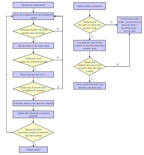
The solution flow of the improved ACO algorithm is shown in Figure 5, and the specific steps of the improved ACO algorithm are as follows.
Step 1, initialize the parameters, including not only the basic parameters of ACO algorithm, but also the pseudo-random factor \(q_{0}\).
Step 2, when \(iter<iter\_ max\) enters the following loop.
Step 3, the kth ant of the population departs from the distribution center.
Step 4, the kth ant selects the next visited node according to the path transfer probability rule, as shown in Eq. 23 or Eq. 24 , and judges whether the node is feasible or not. the feasibility judgment criteria are that the node has not been searched, the current total distance traveled is less than the maximum distance of the vehicle, meets the limit of the maximum number of orders of the vehicle, and meets the service time period of the special node (the customer with a hard time window). if the above conditions are met, the node will be placed in the current taboo table. If the above conditions are met, the node will be placed in the current taboo table; if no node can be found to meet the constraints, then return to the distribution center.
Step 5, determine whether the ant has finished searching all nodes, if so, go to step 6.
If not, return to step four.
Step 6, the next ant starts to visit the node, \(k=k+1\).
Step 7, repeat steps 4, 5 and 6, when each ant has searched all the nodes, it can obtain a number of closed circuits with the distribution center as the starting point and the end point. calculate and save the optimal path and the corresponding optimal value generated by this iteration.
Step 8, using the optimal solution generated from this iteration, globally update the pheromone concentration.
Step 9, when \(iter>iter\_ max\), terminate the operation; otherwise, clear the taboo table and return to step 3 for a new round of iteration.
In order to verify the accuracy of the improved ant colony algorithm in solving the vehicle path problem with capacity, the data set used in this experiment is the CVRP public dataset, which includes the coordinates of the location of the cargo center and each customer point, as well as the load capacity of each vehicle and the demand quantity of each customer point In this paper, we choose 12 CVRP cases for testing, and the experimental environment is CPU for ADM Ryzen 7 4800h with Radeon graphics 2.90 GHZS, and the memory is 8gbgb, and the operating system is 64 Windows 10,and select several data in the test set, including the data of A class and B class which involve fewer customer points and delivery vehicles, and the data of E and P class which involve more customer points and delivery vehicles, of which the data of E class and P class involve more customer points and delivery vehicles. In this paper, 12 CVRP algorithms are selected for testing, from four different criteria: class A, class B, class E and class P. Class A and class B data involve fewer customer points and delivery vehicles, class E and class P data involve more customer points and delivery vehicles, of which the location of the customer points in class E data is more scattered, while the location of the customer points in class P data is relatively concentrated. 210, the initial population size N is 20, the number of selected individuals is 5, the retention probability of elite individuals is 0.25, the crossover probability is [0.5,0.7], the mutation probability is [0.05,0.1], and the number of start iterations g is 0.
The experimental results of the improved genetic algorithm for solving CVRP are shown in Table 1, where distance denotes the distance obtained by the algorithm, PDB denotes the error rate, BS denotes the optimal solution of the algorithm, and AVE denotes the average value obtained by the algorithm for 20 times. it can be seen that when the client nodes are fewer, i.e., the number of nodes is less than 40, the optimal solutions are obtained for all the selected cases, and it can be seen that the improved ant colony algorithm can converge quickly and the number of iteration can be seen that the improved genetic algorithm is able to solve the CVRP quickly. The improved ACO algorithm can quickly converge to the optimal solution. It shows that the improved ACO algorithm has better searching ability, and the average values of class A, B and P problems are closer to the optimal solution, which proves that the algorithm is able to calculate a reasonable driving route when solving small-scale problems. when the number of nodes and delivery vehicles is larger, i.e., the number of nodes is larger than 40, the algorithm’s ability to find the optimal solution decreases, but the error between the optimal solution and known optimal solution is lower than that between the optimal solution and known optimal solution in the selected cases after several iterations. The error between the optimal solution and the known optimal solution of the selected case after several iterations can still be maintained within 1%, and the average error is not more than 1%, so the algorithm is able to find reasonable vehicle distribution routes faster within the acceptable error range.
| Instance | Optimal solution | BS | AVE | The number of iterations in optimal solution | ||
| Distance | PDB(%) | Distance | PDB(%) | |||
| A-n31-k5 | 790 | 790 | 0.0 | 790 | 0.0 | 5 |
| A-n55-k6 | 755 | 755 | 0.0 | 756 | 0.1 | 10 |
| A-n65-k5 | 744 | 743 | 0.1 | 742 | 0.3 | 23 |
| B-n32-k5 | 790 | 790 | 0.0 | 801 | 0.4 | 10 |
| B-n45-k5 | 800 | 800 | 0.0 | 805 | 0.3 | 20 |
| B-n67-k6 | 742 | 742 | 0.0 | 747 | 0.5 | 32 |
| E-n40-k6 | 844 | 844 | 0.0 | 844 | 0.0 | 36 |
| E-n66-k8 | 740 | 751 | 0.5 | 752 | 0.9 | 49 |
| E-n75-k10 | 822 | 831 | 0.5 | 833 | 0.9 | 45 |
| P-n15-k4 | 455 | 455 | 0.0 | 455 | 0.0 | 4 |
| P-n45-k6 | 611 | 615 | 0.1 | 619 | 0.3 | 10 |
| P-n75-k10 | 830 | 836 | 0.3 | 839 | 1.0 | 39 |
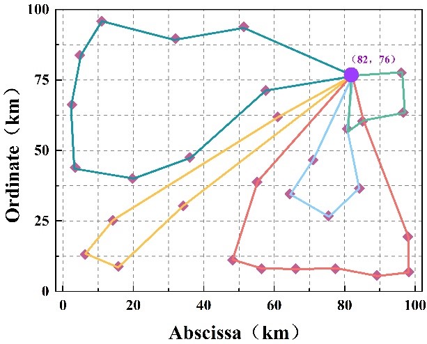
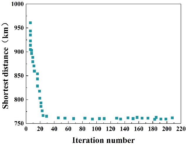
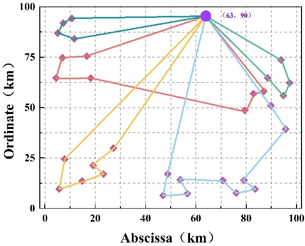
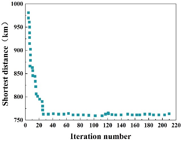
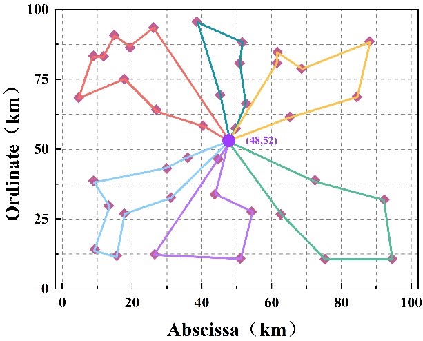
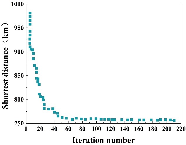
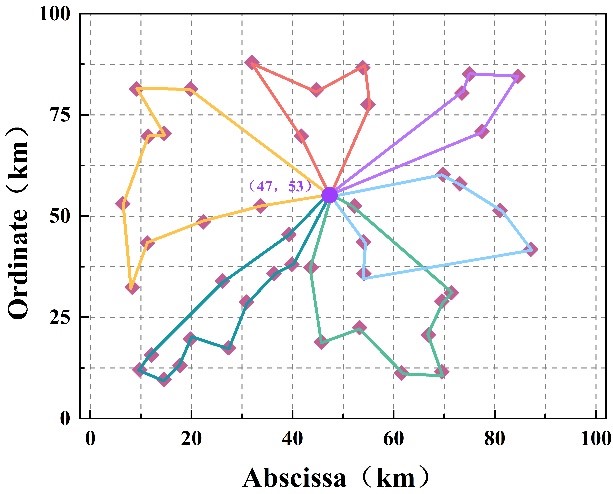
For each type of dataset of A, B, E and P, one instance is selected to draw the optimal path graph and the shortest distance change, and the optimal path graph and the shortest distance change of each type of solution are shown in Figure [f6], in which (a), (b), (c), (d) are the optimal path and the shortest distance change graphs of A-n31-k5, B-n32-k5, E-n40-k6, and P-n45-k6, respectively, and the optimal path and the shortest distance change graphs of the four use cases can be seen by the When there are fewer nodes, i.e. the number of nodes is less than 40, the algorithm can quickly converge to a certain solution, which reflects that the algorithm has a strong global search ability, when there are more client nodes, i.e. the number of nodes is greater than 40, the algorithm objective function value can still fall rapidly before 35 iterations, and the algorithm objective function value can still fall rapidly before 35 iterations, and the algorithm objective function value can still fall rapidly before 35 iterations. When the number of client nodes is more than 40, before 35 iterations, the objective function value of the algorithm is still able to decrease rapidly, and as the number of iterations increases, the value of the objective function decreases gradually, which shows that the algorithm has strong local search ability in the late iteration period. Therefore, the change curve in the above figure shows that the improved ACO algorithm possesses strong global search ability and local search ability, and is able to converge rapidly with a good stability.
In order to further verify the effectiveness of the improved ACO algorithm in this paper, comparative experiments with the same type of solving algorithms are conducted, and the improved firefly algorithm (IFA), simulated annealing algorithm based on large neighborhood search (LNSA) and the traditional ACO algorithm are selected for the experiments, in which “-” indicates that there is no instance solving for this algorithm. A total of 15 instances of different sizes are selected as test sets for three different datasets, A, B, and P. The performance of the different algorithms on various types of data is shown in Table 2.
When solving for all kinds of data, the algorithms for A and B data obtain the optimal solution when the nodes are less than 50, while the improved ACO algorithm is closer to the optimal solution when the nodes are more than 50. For example, the distance of the algorithm is 1779, which is the smallest difference from the optimal solution of 1770 and the PDB is 0.70%, while the PDB of the other algorithms is more than 1.00%. Therefore, the algorithm designed in this paper is feasible and has obvious advantages in solving class A and B data when there are fewer nodes and the location of customers is relatively decentralized or clustered.When solving class P data, the improved ACO algorithm of this paper achieves the optimal solution for all the data at all nodes, and the PDB is 0%, and the optimal solution error of this paper’s algorithm is better than that of the remaining three algorithms.Similarly, in the case of more nodes and relatively centralized location of customers, the distance is 1779, and the difference with the optimal solution is 1770, and the PDB is 0.70%, while the PDB of other algorithms is greater than 1.00%. Similarly, in the case of more nodes and relatively centralized customer location, the algorithm designed in this paper is feasible and can play the biggest advantage, which verifies the effectiveness and robustness of the improved ACO algorithm in this paper.
| Categories | Instance | Optimal solution | IFA | LNSA | ACO | This algorithm | ||||
|---|---|---|---|---|---|---|---|---|---|---|
| Distance | PDB(%) | Distance | PDB(%) | Distance | PDB(%) | Distance | PDB(%) | |||
| A | A-n33-k5 | 650 | 650 | 0.00 | 650 | 0.00 | 650 | 0.00 | 650 | 0.00 |
| A-n48-K5 | 925 | 925 | 0.00 | 930 | 0.45 | 925 | 0.00 | 925 | 0.00 | |
| A-n52-k6 | 1360 | 1361 | 0.06 | 1366 | 0.45 | 1361 | 0.06 | 1360 | 0.00 | |
| A-n67-K8 | 1405 | 1426 | 1.35 | 1426 | 1.35 | 1421 | 1.01 | 1409 | 0.08 | |
| A-n78-k10 | 1770 | 1780 | 1.01 | 1830 | 3.45 | 1822 | 2.90 | 1779 | 0.70 | |
| B | B-n32-k5 | 780 | 780 | 0.00 | 780 | 0.00 | 780 | 0.00 | 780 | 0.00 |
| B-n47-k5 | 830 | 830 | 0.00 | 844 | 0.45 | 830 | 0.0 | 830 | 0.0 | |
| B-n51-k6 | 1600 | 1612 | 0.70 | 1609 | 0.55 | 1603 | 0.05 | 1600 | 0.00 | |
| B-n69-k8 | 1040 | 1050 | 0.95 | 1066 | 2.51 | 1058 | 1.72 | 1046 | 0.41 | |
| B-n79-k10 | 1225 | 1238 | 0.50 | 1242 | 1.02 | 1236 | 0.62 | 1228 | 0.37 | |
| P | P-n30-k5 | 500 | 500 | 0.00 | 500 | 0.00 | 500 | 0.00 | 500 | 0.00 |
| P-n45-k6 | 644 | 644 | 0.00 | 594 | 2.42 | 654 | 1.90 | 644 | 0.00 | |
| P-n58-k8 | 800 | 800 | 0.00 | 812 | 1.82 | 809 | 1.00 | 800 | 0.00 | |
| P-n63-k9 | 795 | 796 | 0.02 | 809 | 1.82 | 803 | 1.03 | 795 | 0.00 | |
| P-n80-k10 | 727 | 728 | 0.15 | 750 | 3.58 | 745 | 2.89 | 727 | 0.00 | |
In order to verify the effectiveness of logistics distribution path optimization based on the improved ACO algorithm in this paper, the e-commerce logistics distribution of Company Z in City X is taken as an example for study. Company Z operates a wide variety of products, including packaged food, daily necessities, cultural and office appliances and clothing, etc. In the mode of transportation, Company Z adopts the three-point-one-line transportation mode of manufacturer-distribution center-distribution station to minimize the intermediate circulation links, and uses refrigerated trucks to transport fresh agricultural products, so as to deliver fresh agricultural products at a faster speed and lower cost. In terms of transportation mode, Company Z adopts the transportation mode of manufacturer-distribution center-distribution station to minimize the intermediate circulating links, and uses refrigerated trucks to transport fresh agricultural and sideline products, so as to deliver the fresh agricultural and sideline products to each store at a faster speed and lower cost.
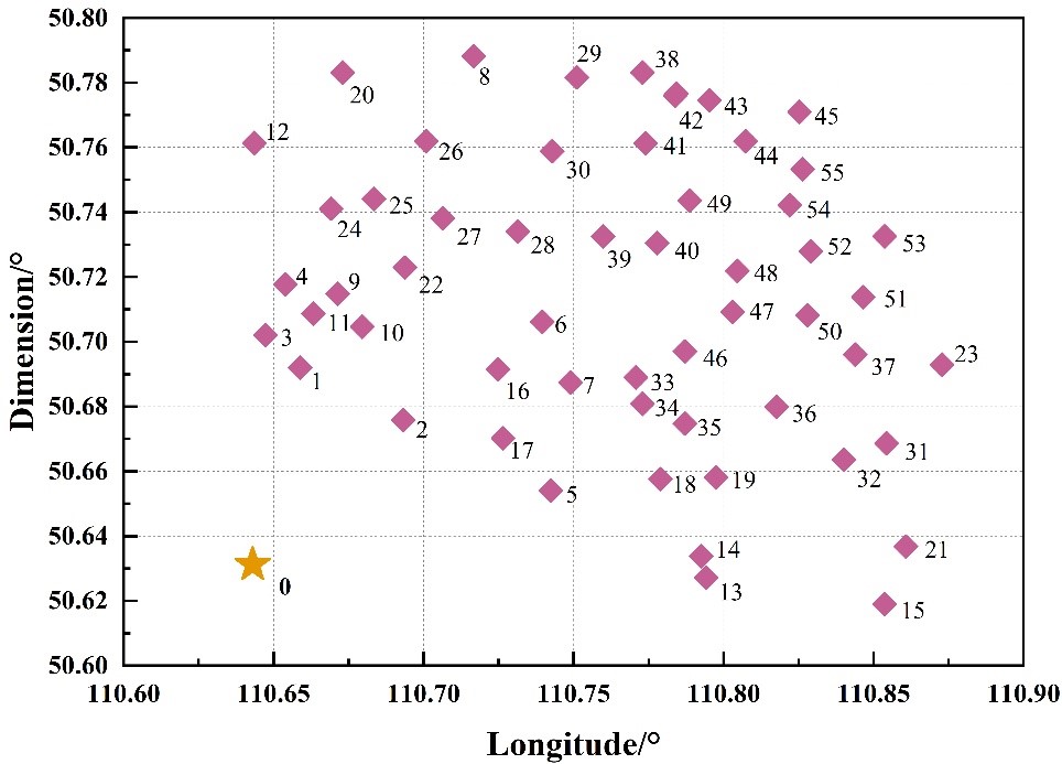
The geographic locations of the distribution center and 55 distribution stations are placed in the latitude and longitude coordinate system, and the distribution center is numbered as P0, and the 55 distribution stations are numbered from 1 to 55, so as to obtain the geographic coordinates of the distribution center and 55 distribution stations. The geographic coordinates of the distribution center and each distribution station are shown in Figure 7, and it can be observed that most of the distribution stations are distributed between 110.70\(\mathrm{{}^\circ}\)\(\mathrm{\sim}\)110.85\(\mathrm{{}^\circ}\) in longitude and 50.70\(\mathrm{{}^\circ}\)\(\mathrm{\sim}\)50.75\(\mathrm{{}^\circ}\) in dimension, and the distribution stations are relatively clustered in comparison with the distribution center, and relatively dispersed among the distribution stations.
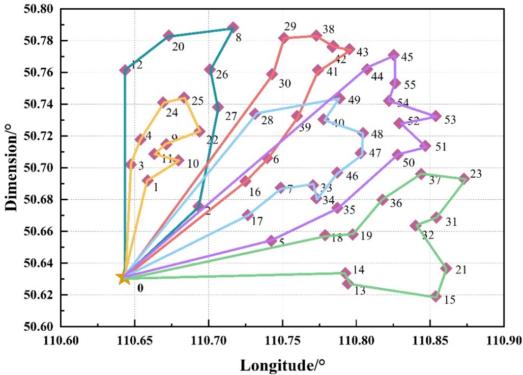
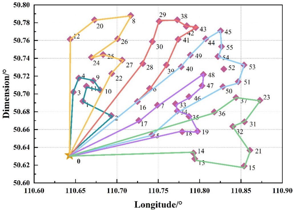
In this experiment, the actual problem of cold chain logistics and distribution of fresh agricultural and sideline products in supermarket Y is transformed into a mathematical model, and the model is simulated using the software, where the total number of ants is set to be two times of the number of supermarket stores, the system constant Q=65, the pheromone function factor \(\alpha\)=1.5, the distance-inspired function factor \(\beta\)=2.5, the time-inspired function factor \(\gamma\)=2, and the pheromone volatile factor \(\rho\)=0.25, and the maximum number of iterations is set to be 150. The e-commerce logistics and distribution optimization problem of company Z under the consideration of the minimum transportation cost is solved six times by using the basic ant colony algorithm and the improved ant colony algorithm in this paper respectively, and the optimal solutions in the results of the six times of the two algorithms are shown in Figure 8, in which (a) and (b) are the path diagrams obtained by the basic ant colony algorithm and the improved ant colony algorithm, respectively. (a) and (b) are the path diagrams of the basic ACO algorithm and the improved ACO algorithm respectively.
It can be seen that the two algorithms are considered the lowest total cost of distribution of the optimal path map is far from each other, but one of the red path, the optimal solution of the basic ACO algorithm is 0-30-29-38-42-43-41-39-6-16-0, while the optimal solution of the improved ACO algorithm is 0-28-30-29-38-42-43-41-39-6-16-0, the optimal solution of the improved ACO algorithm is 0-28-30-29-38-42-43-41-39 -6-16-0,indicating that the optimal solutions of the two algorithms on the red path are approximately the same.
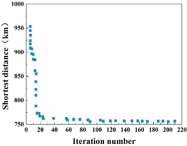
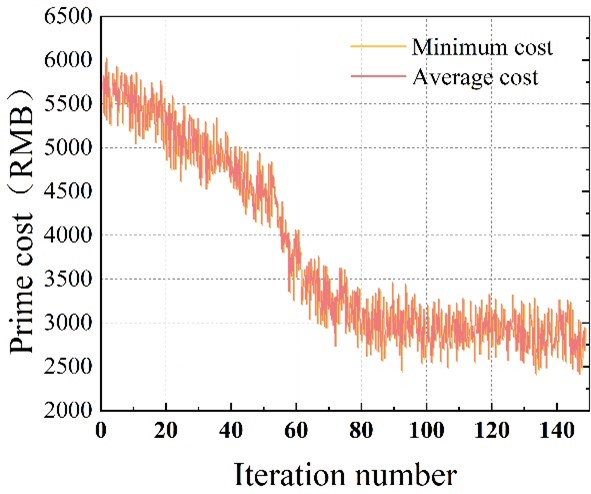
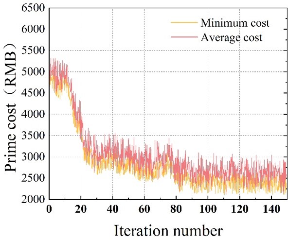
In order to further verify the performance of the two algorithms in the actual analysis, the iterative process of the basic ant colony algorithm and the improved ant colony algorithm are compared and analyzed. The comparison results of the iterative process of the basic ant colony algorithm and the improved ant colony algorithm are shown in Figure [f9], and it can be seen in Figure 9 that, the basic ant colony algorithm is not converged in 80 times of iteration, and the improved ant colony algorithm is faster than the basic one, and in 30 times of iteration, the basic ant colony algorithm converges, and the total cost of searching to the best distribution path is lower. When the number of iterations is 30 times, the algorithm basically converges, and the total cost of searching the optimal distribution path is lower. 70 times of iterations, the minimum cost curve and the average cost curve of the basic ant colony algorithm are only reduced to about 3,000 yuan, while the minimum cost curve and the average cost curve of the improved ant colony algorithm of this paper have been reduced to 2,500 yuan, or even lower, when the number of iterations is 30 times. At the same time, after the convergence of the improved ACO algorithm, the minimum cost curve and the average cost curve do not overlap, this is because the ants of the improved ACO algorithm do not stop searching for other new paths after obtaining the best paths, which improves the stability of the algorithm in obtaining the optimal solution, which indicates that in the actual development of the path optimization, the improved ACO algorithm of the present paper has a better stability of the performance, and has more advantages in its performance.
In order to verify the control of the total cost of transportation in the optimization of e-commerce logistics distribution path by the improved ant colony algorithm of this paper, the total cost of e-commerce logistics distribution after solving the path of the basic ant colony algorithm and the improved ant colony algorithm of this paper are compared and analyzed. The comparison of the total cost of the distribution path of the two algorithms is shown in Table 3, and it can be seen that, the average of the total cost of the basic ant colony algorithm obtained by using the basic ant colony algorithm to solve the path for 6 times is 2976.9 yuan, improve the ant colony algorithm is 2495.8 yuan, improve the ant colony algorithm than the basic ant colony algorithm total cost is lower than 481.1 yuan, reduced by about 16%, at the same time, from the results can also be seen, the basic ant colony algorithm using the number of distribution vehicles is not stable, in the fourth solution used 8 transport vehicles, while improve the ant colony algorithm 5 times the results of the solution are used 6 refrigerated trucks for distribution. For the distribution center, the reduction of the number of distribution vehicles can reduce the labor cost of the distribution center drivers, vehicle repair and maintenance costs, which is conducive to reducing the operating cost of the distribution center. The improved ant colony algorithm can effectively save the total cost of transportation, and carry out scientific and effective distribution path optimization for e-commerce logistics distribution.
| Sequence | 1 | 2 | 3 | 4 | 5 | 6 | Number of vehicles | |
| Basic ant colony algorithm | Number of vehicles | 6 | 7 | 6 | 9 | 7 | 6 | 6.8 |
| Assembly book | 2920.5 | 2870.5 | 3015.8 | 2977.6 | 3040.1 | 3036.9 | 2976.9 | |
| Improved ant colony algorithm | Number of vehicles | 6 | 6 | 6 | 6 | 6 | 6 | 6 |
| Assembly book | 2544.2 | 2540.3 | 2598.8 | 2420.5 | 2452.8 | 2418.5 | 2495.8 | |
| Difference value | 376.3 | 330.2 | 417.0 | 557.1 | 587.3 | 618.4 | 481.1 | |
In this paper, we optimize the distribution path of e-commerce logistics based on the ant colony algorithm, which can effectively deal with the complex path planning problem of e-commerce logistics, and realize the path shortening and cost optimization. in the testing process of several cases, we found that the average distribution distance is reduced by 15%, and the distribution cost is reduced by about 20% after using the ant colony algorithm, which is a remarkable result. This remarkable result comes from the efficient search mechanism and good adaptability of ACO algorithm, which can find the optimal delivery path in the complex e-commerce logistics network.
The application of the algorithm not only improves the delivery efficiency, but also has a significant impact on the reduction of logistics operation costs, which means that e-commerce enterprises can achieve higher cost-effectiveness while ensuring the quality of service. In addition, ant colony algorithm shows stability and extensibility when dealing with large-scale logistics network, indicating that it is suitable for e-commerce enterprises of various sizes. in summary, the ant colony algorithm has a good performance in It not only improves the distribution efficiency, but also significantly reduces the transportation cost, providing an effective optimization tool for e-commerce logistics.
By improving the algorithm of ant colony algorithm, the improved algorithm is applied to solve the problem of logistics vehicle path, and the validity of the algorithm is verified, but there is still some work to be done, and in the actual distribution process, the distribution of the vehicle is often selected according to the type, weight and transport distance of the distribution of the goods. Therefore, the multi-model joint distribution problem can be used as the next research direction.