The pulse propagation that have electromagnetic field inside the optical fiber is controlled by the wave equation, Maxwell’s as shown in Equation 1 . Equations provide as a general model of electromagnetic field transmission through an optical fiber, from which the wave equation [1] can be extracted: \[\label{e1}\tag{1} \bigtriangledown \times \bigtriangledown \times \vec{E}(\vec{r},t)=-\frac{1}{c}\frac{\partial ^{2}\vec{E}(\vec{r},t)}{\partial t^{2}}-\mu_{o}\frac{\partial ^{2}\vec{P}(\vec{r},t)}{\partial t^{2}},\] where \(c\) is velocity of light \(E\) is electric field and \(p\) induce polarization. \[c=\frac{1}{\sqrt{(\mu_0 \epsilon_0 )}},\]
where \(\mu_0\) permabilty and \(\epsilon_0\) permitivity
A phenomenological relationship can frequently be used. However, typically, a quantum-mechanical examination of the link between Er and Pr is necessary as shown in Equation 2 [2]: \[\label{e2}\tag{2} \overrightarrow{P}=\varepsilon_{o}(x^{(1))}\overrightarrow{E}+x^{2}:\overrightarrow{E}\overrightarrow{E}+x^{3}:\overrightarrow{E}\overrightarrow{E}\overrightarrow{E}+…),\]
where the parameter \(X(j)\) is the jth represents the order susceptibility, the term experassion j=1 illustrates the linear relationship. It alters the fiber’s attenuation coefficient and refractive index [3].
Moreover, \(SiO_{2}\) has a small second order susceptibility, which prevents optical fibers from generating second order harmonics. The vulnerability of the third order, \(X^(3)\), is in charge of events like third order harmonic generation, Nonlinear refraction, and four-wave mixing (Kerr effect) [4].
This last result shows how the refractive index fluctuates with intensity, as in Equation 3:
\[\label{e3}\tag{3} \tilde{n}\left( \omega,\left| \overrightarrow{E} \right|^{2} \right)=n(\omega)+n_{2}\left| \overrightarrow{E} \right|^{2}.\]
The value of \(n(\omega)\) expresses the part of the linear effect as contribution, the parameter n2 represents the nonlinear-index part , and related to \(X^{(3)}\).
If nonlinear influences are taken into account, the induced polarization is created by combining two parts: the first part is the linear \(P_{L}(r,t)\), the second part represents the nonlinear part \(P_{NL}(r,t) , P(r,t) = (P_{L}(r,t) + (P_{NL}(r,t)\).
The nonlinear and linear coefficients are related to the electrical field by [5]:
\[\label{e4}\tag{4} \overrightarrow{P_{L}}(\overrightarrow{r},t)=\epsilon_{o}\int_{^{-\infty }}^{\infty }x^{(1)}\left( t-t^{'} \right)\overrightarrow{E}\left( \overrightarrow{r},t^{'} \right)dt^{'}.\]
\[\label{e5}\tag{5} \overrightarrow{P}_{NL}(\overrightarrow{r},t)=\epsilon_{o}\int\int_{}^{}\int_{^{-\infty }}^{\infty }x^{(3)}\left(t-t_{1},t-t_{2},t-t_{3}\right)\vdots \overrightarrow{E}\left( \overrightarrow{r},t_{1} \right)\overrightarrow{E}\left( \overrightarrow{r},t_{2} \right)\overrightarrow{E}\left( \overrightarrow{r},t_{3} \right)dt_{1}dt_{2}dt_{3}.\]
However, the unreliable term is to be considered as a minor a change to the overall polarization to conduct a more condensed analysis. In that regard, it makes sense to start by figuring out how to solve the electrical field in a linear medium.
That is, to take into account the field’s wave equation along the propagation axis \((z)\), in accordance with the analysis as:
\[\label{e6}\tag{6} \tilde{E}_{Z}(\overrightarrow{r},\omega)=A(\omega)F(\rho)e^{\pm im\phi}e^{i\beta z}.\]
Wherein the E field represents the electrionik field, the \(z\) component represents the Fourier transform , A represents the normalization constant, and the parameter \(\beta\) is the constant proliferating and \(m\) is an integer [6].
Additionally, when thinking about the transmission of short pulses, nonlinear effects in optical fibers are especially crucial (from 10ns to 10fs). Both nonlinearities and group-delay dispersion have an impact on the shape and spectrum of these pulses as they pass through the fiber.
According to above analysis, this constructs the wave equation, which takes into account both linear and nonlinear effects [7].
The scalar nonlinear Schrödinger equation (NLSE) can be used to simulate how an electric field propagates in an optical fiber without taking into account polarization [8]:
\[\label{e7}\tag{7} \frac{\partial \tilde{E}(z,t)}{\partial z}=-j\frac{{\beta }_2}{2}\frac{{\partial }^2\tilde{E}\left(z,t\right)}{\partial t^2}+\frac{{\beta }_3}{6}\frac{{\partial }^3\tilde{E}\left(z,t\right)}{\partial t^3}+\frac{g\left(z\right)-\alpha \left(z\right)}{2}\tilde{E}\left(z,t\right)+j\gamma {\left|\tilde{E}\left(z,t\right)\right|}^2\tilde{E}\left(z,t\right).\]
However, it is well known that a wide range of physical phenomena are described by (NLSE), such as modulational instability of the water waves, the movement of a very thin vortex filament in a helical pattern, the transmission of heat pulses in anharmonic crystals, the nonlinear modulation of collisionless plasma waves, and a light beam in a color-dispersive system self-capturing [9].
The nonlinear Schrodinger equation is a general wave equation that first appeared in the research on the propagation of unidirectional wave packets in an energy-efficient, dispersive medium.
The Kerr effect is a feature that occurs in some dielectric components wherein the refractive n index rises according to the electric field’s square. The refractive index can then be expressed as in [10].
A pulse (peak power represent amplitude square, wave, number, and k) moving through a fiber of length L experiences a phase change which is power reliant due to the power dependency of the refractive index [11]:
\[\label{e8}\tag{8} \phi(P)=\phi_{1}+\phi_{nl}=n_{o}kL_{eff}\frac{P}{A_{eff}}m.\]
The Effective length Leff = 1/\(\alpha\) [1-exp(-\(\alpha\) L)] with fiber loss coefficient \(\alpha\) accounts for fiber losses. Howver, both of the polarization properties of the test fiber and the polarization state of signal affect the polarization parameter \(m\).
During the information-processing stage of neural networks, which are made up of trillions of neurons (nerve cells), the exchange of electrical pulses between cells, known as action potentials, takes place. Artificial neural networks (ANNs), which are brain-inspired algorithms, are used to anticipate issues and estimate intricate patterns. The deep learning method, also known as ANN, was founded on the idea that biological neural networks exist in the human brain. ANN was developed in an effort to replicate how the human brain works [12, 13]. Artificial and biological neural networks function in remarkably similar ways, despite certain differences; that is, only structured and quantitative information is accepted by the ANN algorithm.
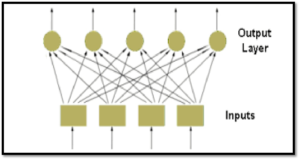
However, in a single-layer feed-forward network, the inputs and outputs are connected by a number of weights in a single layer. Each input is linked to another by weight-carrying synaptic connections.
It is considered to be a feed-forward network, referred to as a “feed-forward system” since information is only transmitted from input to output, as shown in Figure 1.
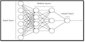
Multiple layers are present in multi-layer feed-forward networks. In addition to input and output layers, this class of networks’ architecture also includes one or more intermediate levels known as hidden layers, as shown in Figure 2.
The field of neural networks has been a significant growth in its applications in fiber optic systems in the recent years. The usage of neural networks is meant to address a wide range of challenges encountered in fiber optic systems, including nonlinear compensation, correction for dispersion of colors and polarization mode divergence.
Several neural network architectures have been used in these applications, such as convolutional neural networks (CNNs), feedforward neural networks, and recurrent neural networks. These architectures have been used to model these defects and improve the performance of optical fiber systems.
It should be noted that although neural networks offer a promising solution to compensate for the nonlinear weakness in optical communication, there are also some limitations to their use. One major limitation is the need for a large amount of data to train the network. In addition, the complexity of the network and the computational resources required can also be limitations. However, despite these limitations, the use of neural networks to compensate for nonlinear weaknesses in visual communication is a promising area of research which is expected to meet a continued growth in the future.
ANN was only utilized as a comparison criterion in this section. As a result, the artificial neural network was used to classify the photos. These photos contain a signal which has been digitally altered using an algorithm like phase-shift keying or quadrature amplitude modulation which is depicted in a constellation diagram. It depicts the signal like a two-dimensional xy-plane scatter diagram in the complex plane at symbol sampling instants
The convolutional neural network (CNN) was used to predict the performance of optic fiber. Table 1 and Figure 3 illustrate the performance of fiber communication system wherein the system enhancement achieved by using intelligent algorithm across fiber channel to reduce the fiber losses. CNN was trained on a dataset (1, 2), representing different parameters such as laser carrier power, data power, fiber nonlinear coefficient, fiber core diameter, refractive index for fiber core and cladding chromatic dispersion, fiber absorption coefficient, and different system parameters. The data set 2 for fiber communication system gives a better performance, as shown in Table 1. The network was able to learn complex nonlinear relationships in the data and to generalize well to unseen measurements of the results for the simulated link seems to have the following parameters with a total length of 400 km of typical single mode fiber, as shown in figures below. \(\gamma\) = 1.2 W/km, \(\alpha\) = 0.2 dB/km, chromatic dispersion CD = 16 ps/nm/km. Moreover, a model for evaluating of simulations was used for various values of fiber.
Table 1 illustrates the results of validation of the first datasets and second dataset.
| Activation Function | First Dataset | Second Dataset |
|---|---|---|
| Saturable A1 | (92 ± 1)% | (99.14±1)% |
| Saturable A2 | (94 ± 1)% | (99±1)% |
| Rectified linear unit | (93.68 ± 1)% | (98.22±1)% |
| hyperbolic tangent | (94.6 ± 1)% | (98.16±1)% |
| Sig.1 | (96.62 ± 1)% | (96.30±1)% |
This compensation will enhance the overall performance system for different bitrate reach to the range from (40 Gb/s -80Gb/s), as shown in Figures 3, 4:
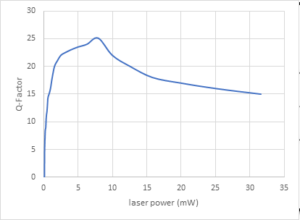
It can be seen that the performance of the system is at data rate 80Gb/s for 400 Km fiber length, as shown in Figure 4:
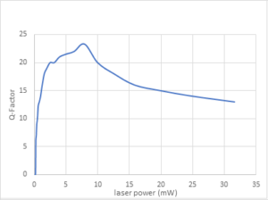
As the need for channel capacity rises, fiber nonlinearity has been discovered to be one of the reasons of limiting the optical fiber systems. This research discusses the way the fiber nonlinearity affects optical fiber system performance. The proposed work produces an efficient fast method for fiber loss compensation. In this method, it can be noted that the fiber system performance at data set 2 with a saturable absorption nonlinear activation function gives preferred performance. This is because the intelligent algorithm can compensate the nonlinear losses, such as nonlinear phase shift and linear losses like absorption and dispersion losses wherein the system reaches up to 80 Gb/s for 400 Km fiber length.