Technological innovation is a hot issue in the present. ESG as the enterprise’s internal strategy has a major impact on the development of enterprise green technology innovation activities. The “dual-carbon” goal is of great significance in promoting the construction of China’s ecological civilization and realizing the goal of modernization of the country, and the report of the twentieth CPC National Congress clearly pointed out that it is necessary to actively and steadily push forward the promotion of carbon peaking and carbon neutrality [1, 2, 3]. Under the direction of “dual-carbon” strategy, we must actively seek a more sustainable way of economic growth, and the concept of corporate ESG refers to the enhancement of corporate sustainability through the integration of environment, society and corporate governance, which is not only a concept of sustainable development, but also a kind of management practice in corporate strategic management [4, 5, 6].
In the process of promoting high-quality economic development in China, it is particularly important to improve the technological innovation ability of enterprises, and from the analysis of the enterprise level, enterprises with innovative ideas pay more attention to creating long-term value rather than obtaining short-term profits, which in turn promotes them to improve their core competitiveness and drive development with innovation [7, 8]. The concept of ESG (Environmental, Social and Governance) encourages companies to consider not only financial data, but also environmental protection, social responsibility, corporate governance and other factors when making business management decisions, so as to comprehensively evaluate the enterprise and make decisions based on it. The concept of ESG has not only attracted the attention of the governmental departments, but has also become a hot spot of research in the academic world [9, 10].
The full implementation of ESG sustainable development strategy is an important driving force to realize the green transformation of economy and society, and an important way to realize the win-win situation of economic development and environmental protection. Budsaratragoon, P., et al. tested the multi-dimensional corporate sustainability and ESG based on the structural equation modeling, and the results showed that social participation is the most important driving force for sustainable development [11]. Röder, J et al. devised a di strict energy system approach for electricity to heat technology, which provides a new research path for solving the problems of unstable power supply and grid congestion [12]. María Cornejo-Caamares, et al. discussed the impact of environmental innovation objectives on marketing and organizational innovation outcomes, and based on a real case study, pointed out that organizational and marketing innovations are positively affected by four environmental objectives [13].
Tolentino, et al. [14] questioned the persistence of the three propositions put forward by Vernon’s product-cycle model, in view of the rapid development of technological capabilities, which have contributed to the establishment and development of emerging economies (multinational corporations) [14]. Zhang, L. et al. conducted an in-depth analysis of the development of green finance in China based on panel cointegration and causality models, and concluded that the technological innovation and development of green finance and HPF are conducive to the fine-tuning of economic globalization [15]. Maldonado, T. et al. pointed out that ACAP is positively correlated to the technological innovation of the organization and the financial performance of the firms, based on 96 related researches and 330 correlation articles [16]. Marin-Garcia, A. et al. proposed a literature-based theoretical model to study the customers of three food retailing formats in an empirical and comparative study, and learned that technological innovation enhances the sustainability of retail development [17]. The study was informed that EKC and LCC are effective, non-renewable energy reduces environmental loads and renewable energy vice versa, and energy technology investment and innovation have no significant effect on ecological footprint and carrying capacity [18]. Deng, X. et al. explored how stock market performance affects firms’ ESG index heterogeneity in different equity contexts, and learned that non-renewable energy sources have no significant impact on ESG indexes [19]. Garcia, A. S. et al. investigated the relationship between corporate finance and good ESG performance in sensitive industries, and pointed out that, regardless of the country and the size, sensitive industries show good ESG performance under political and ethical pressures [20].
This paper uses multiple linear regression model to explore the impact of ESG performance on corporate technological innovation capability. First, Chinese A-share listed companies in Shanghai and Shenzhen are selected from the Wind database as the research sample, and the research database is established by collecting and organizing relevant data. Next, key variables such as ESG performance and corporate innovation are defined and measured, while other variables that may affect the results are controlled. Subsequently, statistical methods are applied to conduct descriptive statistics, correlation analysis and multiple covariance test on the data to ensure the validity of the model. Finally, regression analysis is used to verify the relationship between ESG performance and corporate technological innovation, and robustness tests are used to strengthen the reliability of the research findings.
Let \(y\) be a random variable that can be observed and recorded, and it is obviously influenced by \(m-1\) a non-random factor \(x_{1} ,x_{2} ,\cdots ,x_{m-1}\) and a random factor \(\varepsilon\). There is a relationship between the non-random, random factors and \(y\) based on mathematical and statistical theory, if \(y\) and \(x_{1} ,x_{2} ,\cdots ,x_{m-1}\) have the following linearly related relationship equation; \[\label{GrindEQ__1_}\tag{1} y=\beta _{0} +\beta _{1} x_{1} +\beta _{2} x_{2} +\beta _{m-1} x_{m-1} +\varepsilon,\] where \(\beta _{0} ,\beta _{1} ,\beta _{2} ,\cdots ,\beta _{m-1}\) is the coefficient of the independent variable. The \(\varepsilon\) mean is zero and the variance is \(\sigma ^{2} >0\). It is usually assumed \(\varepsilon \sim N\left(0,\sigma ^{2} \right)\) that the above model is a multiple regression model, where \(y\) is the dependent variable and \(x_{1} ,x_{2} ,\cdots ,x_{m-1}\) is the independent variable.
We first need to make reasonable parameter estimates for the unknown coefficients \(\beta _{0} ,\beta _{1} ,\beta _{2} ,\cdots ,\beta _{m-1}\), so we need to make \(n(n\ge p)\) observations of them first and record them, thus obtaining \(n\) sets of data; \[\label{GrindEQ__2_}\tag{2} \left(x_{i_{1} } ,x_{i_{2} } ,\cdots ,x_{i_{m-1} } ;y_{i} \right)(i=1,2,\cdots ,n).\]
They should satisfy \(y=\beta _{0} +\beta _{1} x_{1} +\beta _{2} x_{2} +\beta _{m-1} x_{m-1} +\varepsilon\), i.e., we have \[\label{GrindEQ__3_}\tag{3} \left\{\begin{array}{l} y=\beta_{0}+\beta_{1}x_{11}+ \beta_{2}x_{12}+\cdots \beta_{m-1}x_{1m-1}+\varepsilon_{1}\\ y=\beta_{0}+\beta_{1}x_{21}+ \beta_{2}x_{22}+\cdots \beta_{m-1}x_{2m-1}+\varepsilon_{2} \\ \vdots \\ y=\beta_{0}+\beta_{1}x_{n1}+ \beta_{2}x_{n2}+\cdots \beta_{m-1}x_{nm-1}+\varepsilon_{n} \end{array}\right.\] where \(\varepsilon _{1} ,\varepsilon _{2} ,\cdots ,\varepsilon _{n}\) are independent of each other and obey a \(N\left(0,\sigma ^{2} \right)\)-distribution.
Let \[\label{GrindEQ__4_}\tag{4} Y=\left[\begin{array}{l} {y_{1} } \\ {y_{2} } \\ {\vdots } \\ {y_{n} } \end{array}\right]_{n\times 1} ,X=\left[\begin{array}{l} {1,x_{1,1} \cdots x_{1,m-1} } \\ {1,x_{2,1} \cdots x_{2,m-1} } \\ {\vdots } \\ {1,x_{n,1} \cdots x_{n,m-1} } \end{array}\right]_{n\times m} ,\beta =\left[\begin{array}{l} {\beta _{0} } \\ {\beta _{1} } \\ {\vdots } \\ {\beta _{m-1} } \end{array}\right]_{m\times 1} ,\varepsilon =\left[\begin{array}{l} {\varepsilon _{0} } \\ {\varepsilon _{1} } \\ {\vdots } \\ {\varepsilon _{n} } \end{array}\right]_{n\times 1}.\]
Then the system of multivariate equations can be abbreviated to the following form; \[\label{GrindEQ__5_}\tag{5} \left\{\begin{array}{l} {Y=X\beta +\varepsilon } \\ {\varepsilon \sim N\left(0,\sigma ^{2} I_{n} \right)} \end{array}\right.\] where \(Y\) is the observed value and \(X\) is the variable observation matrix, which are recorded from the previous data observations, while \(X\) is assumed to be the variable matrix with full rank of columns, i.e., \(r(X)=m\). where \(\beta\) is the column vector of the unknown parameter to be estimated. \(\varepsilon\) is the column vector of random errors that cannot be effectively observed and recorded. The mathematical formula obtained above is the expression of the matrix of the multiple linear regression model and is denoted as \(\left(Y,X\beta ,\sigma ^{2} I_{n} \right)\).
The core problem to be solved for the linear model \(\left(Y,X\beta ,\sigma ^{2} I_{n} \right)\) above is as follows;
Effective estimation of parameters \(\beta\) and \(\sigma ^{2}\) and establishment of the linkage equation between \(y\) and \(x_{1} ,x_{2} ,\cdots ,x_{m-1}\).
The assumptions of the proposed linear model and the assumptions of parameter \(\beta\) can be effectively tested.
Reasonable prediction of the dependent variable \(y\), while the independent variables are effectively controlled and recorded.
As in the case of the simple regression model, the common estimation method for the linear coefficient \(\beta _{0} ,\beta _{1} ,\beta _{2} ,\cdots ,\beta _{m-1}\) in the complex model is still the least squares method, denoted as: \[\label{GrindEQ__6_}\tag{6} Q\left(\beta _{0} ,\beta _{1} ,\cdots ,\beta _{k} \right)=\sum _{i=1}^{N}\left(y_{i} -\beta _{0} -\beta _{1} x_{1i} -\beta _{2} x_{2i} -\cdots -\beta _{k} x_{ki} \right)^{2}.\]
Find its minimum value at point \(\left(\hat{\beta }_{0} ,\hat{\beta }_{1} ,\cdots ,\hat{\beta }_{k} \right)\), i.e., \[\label{GrindEQ__7_}\tag{7} Q\left(\hat{\beta }_{0} ,\hat{\beta }_{1} ,\cdots ,\hat{\beta }_{k} \right)={\mathop{\min }\limits_{\beta _{0} ,\beta _{1} ,\cdots ,\beta _{k} }} Q\left(\beta _{0} ,\beta _{1} ,\cdots ,\beta _{k} \right).\]
Then \(\hat{\beta }_{0} ,\hat{\beta }_{1} ,\cdots ,\hat{\beta }_{k}\) is the least squares estimate of \(\beta _{0} ,\beta _{1} ,\cdots ,\beta _{k}\).
The linear equation for \(\hat{\beta }_{0} ,\hat{\beta }_{1} ,\cdots ,\hat{\beta }_{k}\) is given by the necessary condition for the differential method for the extremum: \[\label{GrindEQ__8_}\tag{8} \begin{array}{l} {\frac{\partial }{\partial \beta _{j} } \sum\limits_{i=1}^{N}\left(y_{i} -\beta _{0} -\beta _{1} x_{1i} -\beta _{2} x_{2i} -\cdots -\beta _{k} x_{ki} \right)^{2} } =0(j=0,1,\cdots ,k) \end{array}.\]
The solution of the Solve this equation and represent it as a matrix; \[\label{GrindEQ__9_}\tag{9} \hat{\beta }=\left(X^{T} X\right)^{-1} X^{T} Y,\] where, \(\hat{\beta }=\left(\beta _{0} ,\beta _{1} ,\cdots ,\beta _{k} \right)^{T}\) and \(X^{T} X\) is required to be invertible.
In this way, the empirical regression equation is obtained as; \[\label{GrindEQ__10_}\tag{10} \hat{y}=\hat{\beta }_{0} +\hat{\beta }_{1} x_{1} +\hat{\beta }_{2} x_{2} +\cdots +\hat{\beta }_{k} x_{k}.\]
As with the simple regression model, Equation \(\sigma ^{2}\) can be estimated, noting; \[\label{GrindEQ__11_}\tag{11} S_{E} =\sum _{i=1}^{n}\left(y_{i} -\hat{y}_{i} \right)^{2} =Q\left(\hat{\beta }_{0} ,\hat{\beta }_{1} ,\cdots ,\hat{\beta }_{k} \right).\]
Then the unbiased estimate of \(\sigma ^{2}\) is, \[\label{GrindEQ__12_}\tag{12} \hat{\sigma }^{2} =\frac{S_{E} }{n-k-1} =\frac{\sum _{i=1}^{n}\left(y_{i} -\hat{y}_{i} \right) }{n-k-1}.\]
Goodness of fit is an identification value used to compare the validity of the regression effect, its size indicates the proportion of the total variance in the response variable that can be explained by the regression equation, \(0\le R^{2} \le 1\), \(R^{2}\) the closer it is to 1, the higher the proportion of the \(Y\) total variance that can be explained by the regression equation, and the more effective it is for prediction. The opposite indicates that it is not applicable for prediction. The value of the goodness of fit also depends on the number of independent variables in the model; an increase in the independent variables does not change the total sum of squares, but increases the regression sum of squares, which means that the denominator remains unchanged, but the numerator becomes larger, and the value of the goodness of fit becomes larger. Which is defined as: \[\label{GrindEQ__13_}\tag{13} R^{2} =\frac{SSR}{SST} =1-\frac{SSE}{SST} =1-\frac{\sum (y-\hat{y})^{2} }{\sum (y-\bar{y})^{2} },\] where \(SSR\) is the regression sum of squares, \(SSE\) is the residual sum of squares, and \(SST\) is the total deviation sum of squares. \(R^{2}\) increase has nothing to do with the goodness of the model, so when there are more independent variables in the model, it is not very appropriate to use the value of the goodness of fit for comparative analysis, in order to eliminate the degree of dependence of the goodness of fit on the number of independent variables in the model, we use the method of correction.
The modified goodness-of-fit formula is; \[\label{GrindEQ__14_}\tag{14} \left\{\begin{array}{rcl} {\bar{R}^{2} } & {=} & {1-\frac{SSE/(n-k-1)}{SST/(n-1)} =1-\frac{SSE}{SST} \cdot \frac{n-1}{n-k-1} } \\ {} & {=} & {1-\left(1-R^{2} \right)\frac{n-1}{n-k-1} } \\ {SST} & {=} & {\sum _{i=1}^{n}\left(y_{i} -\bar{y}\right)^{2} } \end{array}\right.\]
It can be concluded that \(\bar{R}^{2}\) takes into account the average of the residual sum of squares rather than the residual sum of squares itself, and consequently, the larger \(\bar{R}^{2}\) is the better in linear regression modeling predictive analysis.
Let the original hypothesis be \(H_{0} :\beta _{1} =\beta _{2} =\cdots =\beta _{m} =0\) and the alternative hypothesis be \(H_{1} :\beta _{i} ,i=1,2,\cdots ,m\), not all null.
Construct the \(F\) statistic: \[\label{GrindEQ__15_}\tag{15} F=\frac{{SSR\mathord{\left/ {\vphantom {SSR m}} \right. } m} }{{SSE\mathord{\left/ {\vphantom {SSE n-m-1}} \right.} n-m-1} } =\frac{{\sum \left(\hat{y}_{i} -\bar{y}\right)^{2} \mathord{\left/ {\vphantom {\sum \left(\hat{y}_{i} -\bar{y}\right)^{2} m}} \right. } m} }{{\sum \left(y_{i} -\hat{y}\right)^{2} \mathord{\left/ {\vphantom {\sum \left(y_{i} -\hat{y}\right)^{2} \left(n-m-1\right)}} \right. } \left(n-m-1\right)} },\] where \(\sum \left(\hat{y}_{i} -\bar{y}\right)^{2}\) is the regression sum of squares with degrees of freedom \(m\) and \(\sum \left(y_{i} -\hat{y}\right)^{2}\) is the residual sum of squares with degrees of freedom \(n-m-1\). After calculating the \(F\) values from the above equation, the model is tested by checking against the \(F\) distribution table. For the confidence interval \(\alpha =0.05\), the values \(F_{\alpha }\) with degrees of freedom \(m\) and \(n-m-1\) are viewed in the \(F\) distribution table, and if \(F\ge F_{\alpha }\), the existence of a linear correlation between \(y\) and \(x_{1} ,x_{2} ,\cdots ,x_{m}\) is obtained. The converse indicates that the linear correlation between the two is not significant.
Let the original hypothesis be \(H_{0} :\beta _{i} =0\) and the alternative hypothesis be \(H_{1} :\beta _{i} \ne 0,i=1,2,\cdots ,m\).
Construct the statistic; \[\label{GrindEQ__16_}\tag{16} t_{\beta _{i} } =\frac{\beta _{i} }{S_{\beta _{i} } } ,i=1,2,\cdots ,m,\] where \(S_{\beta _{i} }\) is the standard deviation of the regression coefficient \(\beta _{i}\), calculated as: \[\label{GrindEQ__17_}\tag{17} S_{\beta _{i} }^{2} =S^{2} \cdot C_{ii} ,i=0,1,\cdots ,m,\] where, \(S^{2}\) is the regression variance, \(S^{2} =\frac{\sum e_{t}^{2} }{n-k-1}\). \(n\) is the number of observations. \(k\) is the number of independent variables \(C_{ii}\) is the elements on the main diagonal of matrix \(\left(X{'} X\right)^{-1}\), thus \[\label{GrindEQ__18_}\tag{18} S_{\beta _{i} } =\sqrt{S^{2} \cdot C_{ii} }.\]
Based on the given significance level \(\alpha\), the two-sided test for degree of freedom \(n-m-1\) in the \(t\) distribution table is queried to yield the critical value \(t_{\alpha /2} (n-m-1)\).
If \(\left|t_{\beta _{i} } \right|\ge t_{\alpha /2} (n-m-1)\), the original hypothesis \(H_{0}\) is rejected, the regression coefficient \(\beta _{i}\) is not significantly different from 0, and the \(t\) test of the parameter is passed, indicating that it is feasible to choose the independent variable to explain the dependent variable. On the contrary, the original hypothesis cannot be rejected, indicating that the sample observations do not prove that the regression coefficient is significantly different from 0. It means that the \(t\) test of the parameter has not been passed, which indicates that it is not feasible to use the dependent variable to explain the independent variable.
The so-called multicollinearity is to say that the observation and the influence factor are very closely related to each other is not completely unrelated, there is no independent relationship whether it is a single docking or a pair of more than one of the connection is there is a connection, which also shows that this relationship does exist. It is also valid to express the constant relationship as \(b_{0} ,b_{1} ,\cdots ,b_{k}\), \[\label{GrindEQ__19_}\tag{19} b_{0} =b_{1} x_{1} +b_{2} x_{2} +\cdots +b_{k} x_{k}.\] Here for the time being it is determined that a presence \(x_{p}\) can also be shown by other variables as, \[\label{GrindEQ__20_}\tag{20} x_{p} =\frac{a_{0} -\sum _{i\ne p}a_{i} x_{i} }{a_{p} }.\]
From the identification of correlation phenomenon, we can conclude that when calculating the correlation coefficient, if the result is 1, it means that there is a perfect correlation between the two variables. If the result is 0 when calculating the correlation coefficient, it means that the correlation is not perfect and there is some variation, if it is constantly changing between 0 and 1, it also means that there is a correlation between the two variables.
If this property exists for the entire prediction process, then the coefficient \(a_{0} ,a_{1} ,\cdots ,a_{k}\) at partially 0 yields that \(a_{0} =a_{1} x_{1} +a_{2} x_{2} +\cdots +a_{k} x_{k}\) is valid, and from this we utilize the regression coefficients least squares method of estimation \(\hat{\beta }=\left(X{'} X\right)^{-1} X{'} Y\) cannot exist because \(\left(X{'} X\right)^{-1}\) does not exist.
If the whole prediction process exists only approximation of this nature, the existence of the nano-component is partially 0 coefficient \(a_{0} ,a_{1} ,\cdots ,a_{k}\), to get \(a_{0} =a_{1} x_{1} +a_{2} x_{2} +\cdots +a_{k} x_{k}\) is also valid, but then the relative value of \(\left|X{'} X\right|\approx 0\), \(\left(X{'} X\right)^{-1}\) becomes very large, and the relative elements of the variance matrix \(D(\hat{\beta })=\sigma ^{2} \left(X{'} X\right)^{-1}\) of \(\hat{\beta }\) becomes very large, that is to say, the precision of the estimated value may be very low.
The main identifiers are as follows;
mainly through the regression model parameter test as well as equation test to determine, on the one hand, is the team emblem equation of the test with significance that is passed, and the regression model parameter test did not pass, so as to determine that this model has multicollinearity.
in the process of establishing the model needs to be screened whether the selected elements are introduced into the model, in the process of increasing or decreasing each of the factors derived from the model estimates will change, if the change is very obvious that the existence of multicollinearity.
in the process of establishing the regression equation to obtain the corresponding estimated parameters, the estimated parameters obtained by the nature of the actual interest rate with the real life situation to analyze and determine whether it is logical to determine the existence of correlation.
can also determine the degree of correlation between the variables through a simple correlation to determine the extent of correlation, in general, can be used to determine the number of the first relationship, greater than 0.7 can be determined that there is a correlation, with the coefficient of correlation. The problem of multicollinearity exists in practical problems of multiple regression analysis and deserves our attention because it can adversely affect the entire forecasting process.
For example, the quasi-variance of the parameter estimate \(\hat{\beta }\) of the regression equation becomes larger, and this value also indicates whether the goodness of fit of the test is appropriate or not, and also interferes with the relationship.
The larger the variance of the regression coefficients, the weaker the stability of the parameter estimates of the regression equation \(\hat{\beta }\), in the regression coefficients of the test results can be seen in the display of the significance of the test results, if there is a significant means that the test is qualified, but not significant means that the test is unqualified.
The most likely and most concerned problem is the problem of multicollinearity in regression analysis, its adverse effects are very far-reaching and directly affect the prediction of the results of the inaccuracy, we can find out some discriminatory methods to solve the problem, such as intuitive empirical methods, the unit characteristic root method, the method of variance expansion coefficient, and so on.
In this paper, China’s Shanghai and Shenzhen A-share listed companies are selected as the sample, ESG rating data are obtained from Wind database, patent data from iFind Flush database, and all other data from Wind and CSMAR databases. Based on the time interval of the publication of CSM ESG ratings in Wind database, the sample time is chosen as 2005-2022. In this paper, the following treatments are done to the data, excluding financial and real estate industry samples, excluding ST or *ST samples, and excluding samples with missing variables to obtain 28,000 observations. In order to reduce the impact of outliers on the regression results, the continuous variables are shrink-tailed by 1% up and down.
The explanatory variable of this paper is enterprise innovation (EI), patent as the key output of R&D innovation, its application volume can reflect the utilization efficiency of its own inputs, can better reflect the technological innovation ability of enterprises, and is considered to be the core indicator of measuring enterprise innovation. Therefore, this paper uses patent application volume as a proxy variable for innovation. The explanatory variable is ESG performance (HZ_ESG), and this paper chooses the CSI ESG rating to measure the ESG performance of enterprises. The moderating variables are the degree of digital transformation (DCG1) and institutional investor shareholding (Investor). The degree of digital transformation is assessed by summing the logarithms based on the number of times the breakdown of big data technology, cloud computing technology, blockchain technology, artificial intelligence technology, and digital technology applications appear in the annual financial report. This paper also controls for other factors, gearing ratio (LEV), firm size (Size), fixed asset ratio (PPE), profitability level (ROA), tangibility of assets (Tang), sole director ratio (Indep), cash ratio (Cash_Rate), equity concentration (Fhold), capital expenditure ratio (CapEx), operating income growth rate ( Growth), age of the firm (Age), two jobs in one (Merge), and nature of ownership (Soe), with industry, year, and region fixed effects.
This paper analyzes the relationship between ESG performance and corporate technological innovation by introducing the degree of digital transformation and institutional investor shareholding perspectives through a theoretical foundation study. This paper mainly proposes the following hypotheses.
ESG performance can promote corporate innovation.
The degree of digital transformation can positively regulate the relationship between ESG performance and corporate innovation.
Institutional investor shareholding can positively moderate the relationship between ESG performance and corporate innovation.
Table 1 shows the results of descriptive statistics. According to the table, the maximum value of corporate innovation is 7.9677, the minimum value is 0, and the standard deviation is 1.635.The mean value of ESG performance is 4.167, the maximum value is 7, and the minimum value is 1, which indicates that the uneven inputs of different firms in ESG performance lead to a large difference in the ratings obtained. The maximum value of the degree of digital transformation is 5.797, and the standard deviation is 1.398, indicating that the degree of digital transformation varies greatly among listed companies and is unevenly distributed. The mean value of institutional investors’ shareholding is 35.78%, and the maximum value reaches 88.79%, indicating that institutional investors play an increasingly important role in companies.
| Variable | Sample size | Mean | Standard deviation | Minimum value | p50 | Maximum value |
|---|---|---|---|---|---|---|
| EI | 28000 | 3.809 | 1.635 | 0 | 3.892 | 7.9677 |
| HZ_ESG | 28000 | 4.167 | 1.075 | 1 | 4 | 7 |
| DCG1 | 28000 | 1.336 | 1.398 | 0 | 1.078 | 5.797 |
| Investor | 28000 | 35.78% | 24.227 | 0.05% | 35.99% | 88.79% |
| LEV | 28000 | 0.389 | 0.199 | 0.046 | 0.387 | 0.855 |
| PPE | 28000 | 0.218 | 0.196 | 0.005 | 0.189 | 0.6799 |
| Size | 28000 | 22.068 | 1.278 | 19.97 | 21.808 | 26.865 |
| ROA | 28000 | 0.049 | 0.067 | -0.049 | 0.037 | |
| Tang | 28000 | 0.959 | 0.043 | 0.709 | 0.969 | 1 |
| Indep | 28000 | 37.49% | 5.259 | 33.38% | 33.38% | 57.19% |
| Fhold | 28000 | 33.98% | 14.58 | 8.59% | 31.89% | 73.59% |
| Cash_Rate | 28000 | 0.046 | 0.133 | -0.146 | 0.279 | |
| CapEx | 28000 | 0.058 | 0.048 | 0.003 | 0.047 | 0.229 |
| Growth | 28000 | 0.159 | 0.296 | -0.475 | 0.119 | 1.447 |
| Age | 28000 | 1.895 | 0.979 | 0 | 2.068 | 3.278 |
| Merge | 28000 | 0.305 | 0.469 | 0 | 0 | 1 |
| Soe | 28000 | 0.298 | 0.456 | 0 | 0 | 1 |
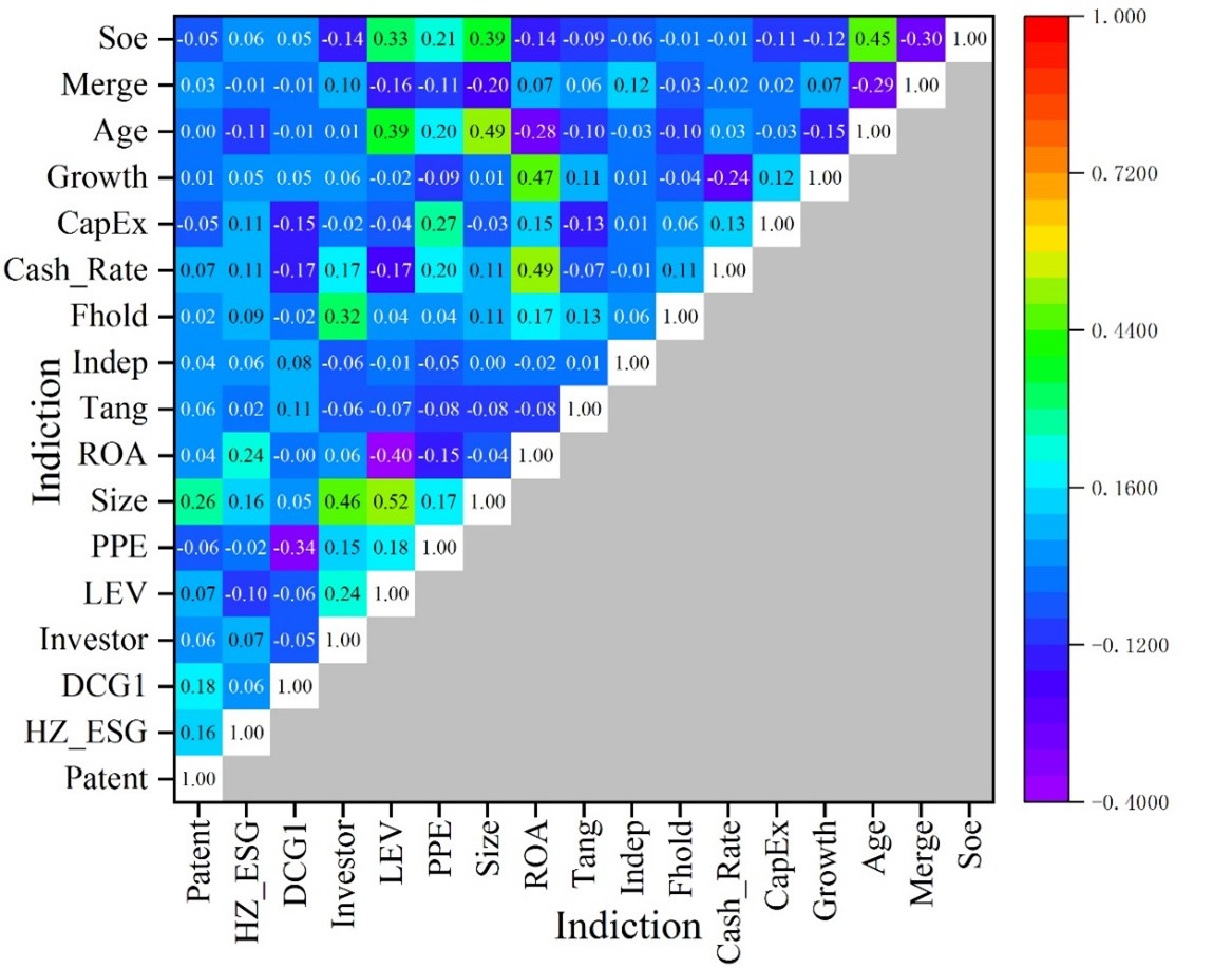
In this paper, Pearson and Spearman correlation tests were conducted to mainly analyze the problem of multicollinearity among the variables. Figure 1 shows the correlation analysis of the indicators. The correlation coefficients between the variables do not exceed 0.8 in absolute value, indicating that there is no highly linear relationship between the variables. Since the correlation analysis can only reveal the variable relationship between two and two, without involving the interactions between the variables, the persuasive power is weak, and this paper also needs to explore the moderating role of the degree of digital transformation, institutional investor shareholding in the relationship between ESG performance and corporate innovation, so it is necessary to do further regression analysis.
Before the regression analysis in this paper, in order to avoid the regression results being affected by the problem of multicollinearity as much as possible, the variance inflation factor is applied, and a further test is made to check whether there is a serious correlation between the variables, and Table 2 shows the test of multicollinearity. The VIF values of all variables are less than 5, and the tolerances are all greater than 0.1, so the correlation between the variables selected in this paper is low, and the results will not be disturbed by the problem of multicollinearity in the next regression analysis.
| Variable | VIF | 1/VIF |
|---|---|---|
| Age | 1.973 | 0.479 |
| Size | 2.019 | 0.507 |
| ROA | 1.841 | 0.479 |
| LEV | 1.737 | 0.555 |
| Investor | 1.568 | 0.589 |
| Soe | 1.545 | 0.673 |
| PPE | 1.439 | 0.686 |
| Cash_Rate | 1.427 | 0.685 |
| Fhold | 1.324 | 0.805 |
| CapEx | 1.280 | 0.794 |
| DCG1 | 1.194 | 0.829 |
| Growth | 1.219 | 0.827 |
| HZ_ESG | 1.104 | 0.865 |
| Merge | 1.109 | 0.874 |
| Tang | 1.082 | 0.968 |
| Indep | 0.985 | 0.996 |
| Mean VIF | 1.458 | |
In order to test the relationship between ESG performance and firm innovation, this paper applies a mixed regression estimation model to regress 28,000 observations. Table 3 presents the basic regression results. Column (1) of Table 3 reports the regression results. The results show that the coefficient between ESG performance and firm innovation is 0.189, which is significantly positive at the 1% level, controlling for control variables and industry, year, and region, suggesting that ESG performance has a positive impact on firm innovation, and that firms with good ESG performance significantly contribute to firm innovation compared to firms with poor ESG performance. So let’s say that A1 is validated. The activities of the esg activities can improve the cognition of the characteristics of the enterprise, strengthen the relationship between enterprises, obtain their support in human, financial and other power and resources, provide guarantee for enterprise innovation, reduce the innovation of enterprises, and do not want to innovate, and enhance the core competitive advantage of enterprises.
Column (2) of Table 3 reports the regression results of the moderating effect of degree of digital transformation. As can be seen from the table, the coefficient of the degree of digital transformation is 0.215, indicating that the degree of digital transformation is an appropriate moderating variable. The coefficient of the interaction term between ESG performance and the degree of digital transformation is 0.028, which is significantly positive at the 1% level, suggesting that the degree of digital transformation strengthens the positive impact of ESG performance on firm innovation and exerts a positive moderating effect between the two. So let’s say that a2 is validated. Digital technology can help enterprises to master user information more accurately, interpret market dynamic demand changes through massive data, provide more accurate and accurate esg information, help enterprises to quickly capture the innovation direction in the process of promoting enterprise innovation, and improve the accuracy of development technology innovation projects.
Table 2, column (3) shows the results of institutional investors’ shareholding as a moderating variable, the coefficient of the interaction term between ESG performance (HZ_ESG) and institutional investors’ shareholding is 0.002, which is significantly positive at the 10% level, which indicates that institutional investors’ shareholding is able to positively regulate the relationship between ESG performance and corporate innovation, and that it is able to exert a significant moderating effect. So let’s say that A3 is validated.
Institutional investors based on supervisoryism will pay more active attention to corporate development and deeply participate in corporate governance in order to pursue stable returns. They bring their core competence in professional investment and research to corporate governance, and are committed to creating a benign environment suitable for ESG development, so that companies can focus on innovation to enhance and maintain their competitive advantages and realize sustainable development. In addition, institutional investors will force management to accept their own ESG-related decision-making concepts by virtue of their gradually increasing shareholding, urge management to implement ESG concepts, improve ESG performance, and reduce managers’ short-sighted behavior towards R&D and innovation.
| Variable | (1) | (2) | (3) |
|---|---|---|---|
| EI | EI | EI | |
| HZ_ESG | 0.189*** | 0.176*** | 0.185*** |
| (20.56) | (19.49) | (20.45) | |
| DCG1 | 0.215*** | ||
| (27.54) | |||
| HZ_ESG_DCG1 | 0.028*** | ||
| (4.76) | |||
| Investor | 0.002* | ||
| (1.94) | |||
| HZ_ESG_Investor | 0.003*** | ||
| (5.68) | |||
| LEV | 0.508*** | 0.513*** | 0.526*** |
| (8.12) | (8.26) | (8.38) | |
| PPE | -1.158*** | -0.719*** | -1.148*** |
| (-15.29) | (-9.36) | (-15.25) | |
| Size | 0.348*** | 0.315*** | 0.336*** |
| (30.76) | (28.73) | (29.46) | |
| ROA | -0.858*** | -0.629*** | -0.842*** |
| (-4.49) | (-3.36) | (-4.39) | |
| Tang | 1.798*** | 1.549*** | 1.818*** |
| (8.69) | (7.49) | (8.69) | |
| Indep | 0.001 | -0.0003 | 0.001 |
| (0.89) | (-0.08) | (0.86) | |
| Fhold | 0.001* | 0.003*** | 0.001 |
| (1.96) | (2.67) | (1.39) | |
| Cash_Rate | 1.286*** | 1.268*** | 1.249*** |
| (8.29) | (8.29) | (7.98) | |
| CapEx | -0.902*** | -0.869*** | -0.919*** |
| (-4.49) | (-4.36) | (-4.55) | |
| Growth | -0.109*** | -0.126*** | -0.109*** |
| (-3.16) | (-4.08) | (-3.29) | |
| Age | -0.085*** | -0.096*** | -0.096*** |
| (-6.42) | (-7.53) | (-7.14) | |
| Merge | 0.036* | 0.025 | 0.039* |
| (1.88) | (1.19) | (1.78) | |
| Soe | -0.119*** | -0.075*** | -0.119*** |
| (-4.46) | (-2.89) | (-4.56) | |
| Constant | -7.883*** | -7.139*** | -7.669*** |
| (-25.59) | (-23.36) | (-24.68) | |
| N | 28000 | 28000 | 28000 |
| R-squared | 0.275 | 0.295 | 0.276 |
| r\({}^{2}\)_a | 0.274 | 0.294 | 0.275 |
| Ind | Yes | Yes | Yes |
| year | Yes | Yes | Yes |
| area | Yes | Yes | Yes |
In order to further validate the accuracy and improve the credibility of the conclusions of this paper, the following robustness tests are carried out in this paper, endogeneity test by PSM propensity score matching method and instrumental variables method, and other robustness tests are mainly carried out from the transformation of the explanatory variables measure, and lag one period of the explanatory variables.
Compared with enterprises with poor ESG performance, enterprises with good ESG performance may have the advantage of technological innovation themselves and actively engage in technological innovation activities. The conclusion may be affected by the self-selection of the sample, so the PSM propensity score matching method is used to narrow down the impact of differences in the characteristics of the sample enterprises on the conclusion.
In this paper, the industry annual median of the explanatory variable ESG performance is used as the critical value to construct a dummy variable, and the sample group with better ESG performance is set as the experimental group, and the sample group with worse ESG performance is set as the control group. All control variables in the original model are regressed against the dummy variables to derive a propensity score for each observation. Table 4 shows the PSM balance test. The samples were matched using the radius matching method, and the total number of matched samples was 27,888 without significant shrinkage. Table 4 shows the results of the PSM balance test, U indicates before performing the matching, M indicates after performing the matching, after matching the experimental group and the control group are not significant on the control variables, and the rate of deviation of the variables after matching is within 5%, which indicates that PSM is effective and feasible, and the problem of sample self-selection can be controlled to some extent.
| Variable | UnMatchedMatched | Mean | %bias | %reduct bias | t-test | ||
|---|---|---|---|---|---|---|---|
| Treated | Control | t | p\(\mathrm{>}\)t | ||||
| LEV | U | 2.472 | 2.411 | 4.861 | 1.170 | -0.98 | 0.217 |
| M | 2.592 | 2.536 | -1.568 | 66.393 | 0.547 | ||
| PPE | U | 24.059 | 24.102 | -2.465 | -0.592 | 0.56 | 0.491 |
| M | 24.055 | 23.968 | 1.626 | 39.028 | 0.603 | ||
| Size | U | 0.475 | 0.466 | -4.117 | -1.046 | -0.47 | 0.330 |
| M | 0.492 | 0.412 | -1.455 | 65.354 | 0.501 | ||
| ROA | U | 0.052 | 0.099 | -3.869 | -1.053 | -0.09 | 0.306 |
| M | 0.133 | 0.142 | -0.052 | 98.353 | 0.904 | ||
| Tang | U | 0.076 | 0.032 | -1.742 | -0.452 | -0.17 | 0.664 |
| M | 0.104 | 0.063 | -0.302 | 79.551 | 0.974 | ||
| Indep | U | 0.561 | 0.666 | -5.231 | -1.428 | -0.18 | 0.184 |
| M | 0.693 | 0.679 | -0.407 | 92.186 | 0.897 | ||
| Fhold | U | 0.435 | 0.378 | 5.026 | 1.318 | -0.98 | 0.232 |
| M | 0.434 | 0.266 | -2.841 | 43.994 | 0.361 | ||
| Cash_Rate | U | 0.514 | 0.372 | 7.530 | 1.961 | 0.57 | 0.001 |
| M | 0.340 | 0.345 | 1.589 | 78.275 | 0.569 | ||
| CapEx | U | 0.140 | 0.288 | -19.678 | -5.351 | 0.18 | 0.060 |
| M | 0.155 | 0.205 | 0.340 | 98.058 | 0.935 | ||
| Growth | U | 0.489 | 0.321 | 13.250 | 3.445 | 1.09 | -0.073 |
| M | 0.415 | 0.499 | 3.015 | 76.361 | 0.356 | ||
| Age | U | 0.477 | 0.420 | 13.269 | 3.482 | 1.05 | -0.017 |
| M | 0.529 | 0.462 | 3.066 | 76.289 | 0.240 | ||
| Merge | U | 0.512 | 0.450 | 13.388 | 3.428 | 1.03 | -0.021 |
| M | 0.518 | 0.533 | 3.058 | 76.317 | 0.260 | ||
| Soe | U | 0.452 | 0.433 | 13.255 | 3.495 | 1.05 | 0.048 |
| M | 0.581 | 0.479 | 3.137 | 76.367 | 0.263 | ||
The new samples after matching are regressed again, and Table 5 shows the regression results of PSM propensity score matching test. From the PSM propensity score matching regression results, it can be seen that the correlation coefficients between ESG performance and the degree of technological innovation and digital transformation of enterprises are still significantly positive, and the correlation coefficients are 0.044 and 0.001, respectively. The degree of digital transformation still plays a partly intermediary role in the promotion of the technological innovation activities by the ESG performance of enterprises.
| (1) | (2) | (3) | |
|---|---|---|---|
| EI | DCG1 | EI | |
| ESG | 0.045* | 0.001** | 0.044* |
| (1.959) | (1.989) | (1.922) | |
| DCG1 | 1.754** | ||
| (2.478) | |||
| Investor | 1.595** | ||
| (2.298) | |||
| LEV | 0.042 | 0.002*** | 0.039 |
| (1.250) | (3.094) | (1.149) | |
| PPE | -0.580*** | -0.129 | -0.580*** |
| (-22.937) | (-0.206) | -23.049 | |
| Size | 0.555*** | -0.007* | 0.566*** |
| (3.67) | (-1.667) | -3.742 | |
| ROA | -0.018 | -0.064*** | -0.118 |
| (-0.088) | (-6.769) | -0.534 | |
| Tang | -1.120*** | 0.076*** | -1.238*** |
| (-2.842) | -6.384 | (-3.078) | |
| Indep | 0.301*** | 0.001 | 0.299*** |
| (4.891) | (0.861) | (4.87) | |
| Fhold | 0.063 | 0.022*** | 0.028 |
| (0.167) | (2.609) | (0.075) | |
| Cash_Rate | -0.009 | -0.010*** | 0.008 |
| (-0.059) | (-3.399) | -0.052 | |
| CapEx | -0.113** | -0.003** | -0.107* |
| (-2.015) | (-2.305) | (-1.923) | |
| Growth | -0.106** | -0.007*** | -0.118** |
| (-2.037) | (-6.875) | (-2.24) | |
| Age | -13.587*** | -0.052*** | -13.667*** |
| (-23.848) | (-3.979) | (-23.992) | |
| Merge | -0.087 | 0.015*** | 0.006 |
| (-0.047) | (-3.677) | (0.068) | |
| Soe | -0.197** | -0.069** | -0.179* |
| (-2.956) | (-2.897) | (-1.658) | |
| Industry | 0.799** | 0.899*** | 0.758** |
| (2.868) | (6.798) | (2.789) | |
| Constant | -0.079 | -0.019*** | 0.869 |
| (-0.289) | (-3.398) | -0.097 | |
| Year | Yes | Yes | Yes |
| Ind | Yes | Yes | Yes |
| Area | Yes | Yes | Yes |
| N | 27888 | 27888 | 27888 |
| F | 116.388 | 16.437 | 113.876 |
| Adj_R\({}^{2}\) | 0.517 | 0.184 | 0.518 |
ESG performance and firms’ technological innovation activities may be endogenous with reverse causality, i.e., firms with active technological innovation activities are more likely to disclose ESG information and have good ESG performance. In this paper, 2SLS regressions are conducted using the mean ESG value (Mesg) of firms in the same industry as an instrumental variable. Table 6 shows the 2SLS regression results. On the one hand, after the weak correlation test, the correlation between Mesg and the explanatory variables is strong, and the ESG means of firms in the same industry fulfill the correlation requirement. On the other hand, the ESG mean values of other enterprises within the same industry cannot have an impact on the green technology innovation activities of this enterprise, and the instrumental variables are not correlated with the random disturbance term. Therefore, the instrumental variable selection is reasonable.2 the results of the SLS regression are shown in Table 6, ESG performance is significantly and positively correlated with firms’ technological innovation, and the correlation coefficient between Hz_ESG and firms’ technological innovation is 0.268, and it is positively correlated at the 1% level. Consistent with the previous findings, therefore the endogeneity problem due to mutual causation has no decisive influence on the conclusions of this paper.
| (1)ESG | (2)EI | |
|---|---|---|
| Mesg & 0.969*** & | ||
| & (9.675) & | ||
| Hz_ESG | 0.268** | |
| & | (2.099) | |
| LEV | 0.028 | 0.0417 |
| (0.826) | (1.273) | |
| PPE | -0.179*** | -0.559*** |
| (-9.385) | (-17.159) | |
| Size | 0.096*** | 3.705*** |
| (0.623) | (0.179) | |
| ROA | -0.609*** | -0.906*** |
| (-0.077) | (-0.830) | |
| Tang | 0.25*** | 0.29*** |
| (2.866) | (2.234) | |
| Indep | 0.079* | 0.279*** |
| (1.668) | (4.646) | |
| Fhold | 0.606** | 0.239 |
| (2.389) | (0.679) | |
| Cash_Rate | 0.299** | 0.269* |
| (2.498) | (1.825) | |
| CapEx | -0.226*** | -0.223*** |
| (-5.746) | (-3.899) | |
| Growth | -0.118*** | -0.085 |
| (-2.985) | (-1.589) | |
| Age | -0.292** | -0.260* |
| -2.499 | (-1.857) | |
| Merge | 0.256*** | 0.257*** |
| (5.747) | (3.574) | |
| Soe | -0.146*** | -0.057 |
| (-2.957) | (-1.586) | |
| _Cons | -4.197*** | -13.688*** |
| (-6.709) | (-25.976) | |
| Year | Yes | Yes |
| Industry | Yes | Yes |
| Area | Yes | Yes |
| N | 27888 | 27888 |
| F | 28.035 | 123.815 |
| Adj_R\({}^{2}\) | 0.279 | 0.5976 |
Based on the observations of 28,000 Shanghai and Shenzhen A-share listed companies, this paper analyzes the relationship between ESG performance and corporate technological innovation capability in depth using multiple linear regression models. It is found that firms with good ESG performance are more capable of promoting technological innovation, and the correlation coefficient between ESG performance and corporate innovation is statistically significantly positive (0.189, p\(\mathrm{<}\)0.01). This suggests that firms that invest in environmental protection, social responsibility and good governance are more inclined to adopt innovative strategies, which in turn promotes their long-term sustainability.
In terms of moderating variables, the degree of digital transformation and the presence of institutional investor holdings significantly reinforce the positive impact of ESG performance on corporate innovation. Digital transformation provides new opportunities and challenges for firms to innovate, while institutional investor shareholding contributes to a greater focus on innovation and sustainability by strengthening corporate governance and strategic planning.
Robustness tests further confirm this finding through the PSM propensity score matching method and the instrumental variables method, which demonstrates that the positive association between ESG performance and firms’ technological innovation remains solid even after controlling for sample selection bias. The instrumental variables method excludes potential reverse causality and confirms the positive impact of ESG performance on firms’ technological innovation.
The results of the study emphasize the important role of ESG in promoting technological innovation in enterprises and provide valuable insights for business managers and policy makers. Enterprises should actively invest in ESG-related activities, increase digital infrastructure construction and digital R&D investment and the introduction of digital high-end talents in order to promote technological innovation and achieve long-term sustainable development. At the same time, enterprises should proactively attract institutional investors and take advantage of their strong resources to obtain financial and material support for them to promote ESG practices and facilitate their innovative development.
ESG performance will be an important measure of enterprise technological innovation, and the future can be further studied in different industries, different companies, and technology innovation.