1. Introduction

ubdivision surfaces were introduced in the late 1970’s in computer aided design. SD techniques are the essential tools that helps in the formation of smooth curves and surfaces. These help us to generate new shapes and curves with the help of the sets of control points that vary. It is an innovative technique that is used for the generation of the smooth surfaces as a sequence of successively refined polyhedral meshes. These SD techniques are currently extensively used in various fields such as computer graphics, solid modeling, computer game software, film animations and so on.

The idea to generalize a four-point SD technique to an interpolating SD technique came in 1990, described by Dyn, Gregory and Levin. An interpolating technique was at first defined over a triangular grid. A method is interpolating if the initial and all the subsequent generated control points remains in the mesh as the SD process proceeds. An approximating subdivision scheme was first introduced over a quadrilateral grid by Catmull and Clark in 1978. A process is called approximating if the limit curve includes only the newly generated control points. At each refining step the old control points get excluded. A SD technique is recursive in nature. The process of SD starts with initial polygon having discrete representation and then continues resulting in a smooth limiting curve. The existence of limit curves and their properties had to be introduced from the given finite number of coefficients, known as the generated mask of the SD technique, that defines the SD refinement rule. A repeated application of the SD rules generates the smooth surface, the process of refinement helps in how to add new vertices and averaging in where to add the new vertices. After the infinite number of refinements applied, a limit surface (or curve) is obtained. This curve is in much refined form as compared to the initial polygon. The analyzation of a non-stationary SD techniques includes a fixed refinement rules applied on a given set of points, but with the change in each refinement level, new points were introduced. The analysis of convergence is done by comparing the given technique with converging stationary SD technique, and similarly the analysis of smoothness is related to the derived first divided difference technique in stationary case. Similarly, by using the respective symbols and the z-transforms of given control points, it is possible to evaluate the convergence and smoothness of SD technique by simple algebraic operations.

SD techniques are iterative formulas for creation of smooth bends/ surfaces. These techniques lately turned into a fundamental piece of Computer aided designs. CAGD is basis tool that displays an art and respective data efficiently and expressively to the observer. It manages the scientific portrayal of shapes for use in Computer illustrations, numerical examination and estimate hypothesis. It is also helpful for processing image data received from the physical world.

P. Novara and L. Romani [1] exhibited 3 parameter joined ternary 4-to point subdivision conspire that gives a binding together system to a few autonomous propositions showed up in the writing. Z. Luo and W. Qi [2] utilized the technique for deducting interpolatory from approximating SD plot. S. Lin et al. [3] introduced another insertion subdivision plot for blended triangle/quad networks that is C1 continuous. C. Conti et al. [4] presented another proportionality idea among non-stationary SD plans named asymptotically likeness which is flimsier than asymptotically identicalness is presented and contemplated. J.Q Tan et al. [5] displayed another paired four-point SD plot which maintains the second control isolated contrast at the ancient apexes unaltered when the starting apexes are embedded. S.S Siddique et al. [6] displayed binary 3-point and 4-point non-stationary plans utilizing hyperbolic capacities as premise capacities. S.S. Siddique and M. Younis [7] built up a calculation to build m point (for any whole numbers) binary approaching SD plans utilizing Cox-de Boor recursion formula. S.S. Siddique and K. Rehan [8] improved a binary four-point resembling SD plot exhibited by Siddique and Ahmed (2006) by presenting worldwide tension parameter. G. Mustafa et al. [9] used the least quadrangles system for (2n)²-perceptions to fit berate cubic paranormal for \(n\geqslant 2\). G. Mustafa and R. Hameed [10] exhibited the groups of parameters subordinate univariate and bivariate SD plans. G. Mustafa and M. Bari [11] introduced varied extending groups of SD plans for suitable information to SD models. P. Novara and L. Romani [12] characterized the structure squares to acquire new groups of non-stationary SD plans. Bashir et al. [13] managed general methods of parameterized and non- parameterized bivariate SD plot with four parameters. M. Bari et al. [14] defined a method that is used to develope 3n-point quaternary approximating subdivision techniques. S.S. Siddique and T. Noreen [15] analyzed the property for six-point ternary interpolating subdivision technique that preserve convexity. H. Zheng and B. Zhang [16] presented a non-stationary combined subdivision technique that combines several approximating and interpolating subdivision techniques. P. Novara et al. [17] constructed a non-stationary subdivision scheme having several properties for 3 directional grids. M. Asghar et al. [18] introduced a simple way to increase the continuity of the subdivision schemes. G Kanwal et al. [19] developed a new numerical technique that defines a 6-point approximating subdivision techniques that helps in the generation of the smooth curves. S. A. Manan et al. [20] defines a technique to get the solution of 3^rd order BV problem that is approximating 8-point scheme. G. Mustafa and S.T. Ejaz [21] introduced the two scale relation derivatives that are fulfilled by the subdivision technique and then used these results to construct the new subdivision method. G. Mustafa et al. [22] proposed a new iterative numerical approach that depends on interpolating subdivision techniques which gives the solution of four-point boundary value problems. G. Mustafa and R. Hameed [23] presented univariate and bivariate subdivision schemes forming families of parameter. J. Tan et al. [24] presented a non-stationary approximating 3-point SD scheme that helps in the generation of an vast variety of C³ continuous limit curves. L. Romani [25] presented a parameter-dependent RS subdivision algorithm. The newly generated C⁴ approximating subdivision technique has a wide range continuity that is broadly used in the field of geometric representations, movement and animations. For more details on C⁴ approximating subdivision technique, we refer the readers to [26–32].

2. Stationary Four-Point Technique

A combined four-point SD technique generate C⁴ limiting curve. We are initially given the control set points \(s^{0} = \{{s_{i}^{0}\}}_{i \in z}\) at level 0, with the help of which we have to generate the new control points \(\{{s_{i}^{k + 1}\}}_{i \in z}\) at an optimized level k+1 using the SD technique. \[s_{2i}^{k + 1} = \left( \frac{1}{8} – \gamma \right)s_{i – 1}^{k} + \ \left( \frac{3}{4} + 2\gamma \right)s_{i}^{k} + \left( \frac{1}{8} – \gamma \right)s_{i + 1}^{k},\] \[\label{1}\tag{1} s_{2i + 1}^{k + 1} = \delta s_{i – 1}^{k} + \left( \frac{1}{2} – \delta \right)s_{i}^{k} + \left( \frac{1}{2} – \delta \right)s_{i + 1}^{k} + \delta s_{i + 2}^{k},\] where \(\gamma\) and \(\delta\) are the real constants.

Now, if we take \(\gamma\)= -2\(\delta\), we get the new control points as \[s_{2i}^{k + 1}= (\frac{1}{8} + 2\delta){\ s}_{i – 1}^{k} + (\frac{3}{4} – 4{\delta)\ s}_{i}^{k} + (\frac{1}{8} + 2{\delta)\ s}_{i + 1}^{k},\] \[\label{2}\tag{2} s_{2i + 1}^{k + 1}= \delta s_{i – 1}^{k} + \left( \frac{1}{2} – \ \delta \right)s_{i}^{k} + \left( \frac{1}{2} – \delta \right)s_{i + 1}^{k} + {\delta s}_{i + 2}^{k}\ ,\] which is also combined one and \(\gamma\) being the real constant.

3. The C^l Convergence

In respective section, we are going to deal with the C^l convergence of the above-mentioned combined technique (2). To get the C^l convergence of the combined SD technique (2), let us discuss the respective results:

4. Non-stationary Four-Point SD Technique

A non-stationary four-point SD technique is described by the refinement rules defined in section 2, since the respective control set points are defined as \[s_{2i}^{k + 1}= a_{0}^{k}s_{i – 1}^{k} + a_{1}^{k}{\ s}_{i}^{k} + a_{2}^{k}s_{i + 1}^{k},\] \[\label{3}\tag{3} s_{2i + 1}^{k + 1}= a_{3}^{k}s_{i – 2}^{k} + a_{4}^{k}s_{i – 1}^{k} + a_{5}^{k}\ s_{i}^{k} + a_{6}^{k}s_{i + 1}^{k},\] where \(s^{{^\circ}} = {\{ s_{i}^{0}\}}_{i \in Z}\) is the set of initial control points at very first level 0 and satisfies the relation \(a_{0}^{k} + a_{1}^{k} + a_{2}^{k} = 0\) and \(a_{3}^{k} + a_{4}^{k} + a_{5}^{k} + a_{6}^{k} = 0\) similarly.

The coefficients of a non-stationary SD technique are given by \[\begin{split} & a_{0}^{k}=\ \frac{1}{8} + 2s\left( \delta^{k + 1} \right) = a_{2}^{k}, a_{1}^{k}=\ \frac{3}{4} – 4s(\delta^{k + 1}),\\ & a_{3\ }^{k}=\ s(\delta^{k + 1})=a_{6}^{k}, a_{4}^{k}\ = \frac{1}{2} – s\left( \delta^{k + 1} \right) = a_{5}^{k}, \end{split}\] \[\label{4}\tag{4} s{(\delta}^{k + 1}) = \frac{1}{2\lbrack\left( \delta^{k + 1} \right)^{2} – 9\rbrack},\] with \[\label{5}\tag{5} \delta^{k + 1} = \sqrt{\delta^{k} + 20}, \beta^{0} \in \lbrack – 20, – 11) \cup ( – 11, + \infty).\] The coefficients {\(a_{i}^{k}\}\) thus be calculated at each arbitrary level k, where the initial parameter lies within domain \(\delta^0 \in [-20,-11) \cup (-11,\infty)\).

This must be noted that, starting from any \(\delta^0 \geq20\), we have \(\delta^0 +20 \geq 0, \forall k\in Z+\), so \(\delta^{k+1}\) is always well defined. Obtaining such a wide variety of definition enables us to achieve significant changes in structures of the limit curves.

5. Smoothness Analysis

Here we do the convergence analysis of a non-stationary four-point SD technique Eq. 3 which generates C⁴ continuous limit curves for every value of the initial tension \(\delta^{0}\) in its respective domain provided in Eq. 5.

Basis Function

Basis function is defined as a limit function for initial data. The basis function of order one has the form:

\[n{[}x{]}= \left\{ \begin{matrix} 1\ &\text{if}\ 0 \leq x \leq 1 \\ 0\ &\text{otherwise}. \\ \end{matrix} \right.\ \ \]

This function is zero everywhere except where it is constant. i.e. [0,1)

7. Graphical view

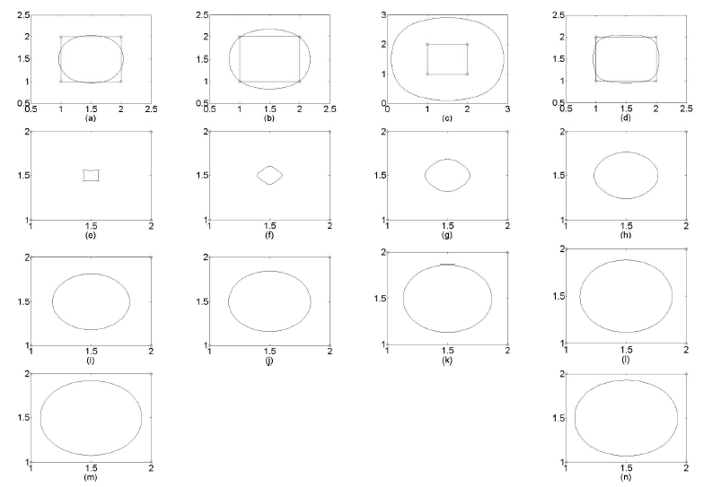
In this respective section, we are now going to discuss the behavior of a proposed technique (5) considering an example. As discussed earlier in case (3.2) from inwards to outwards behavior of a discrete polygon as \(\delta^{0}\rightarrow \infty\).

In Figure (1), the geometric behavior of a non-stationary combined four-point subdivision technique is elaborated that generates C⁴ continuous limit curves for the wide range of C⁴ limiting curve using the formulated technique (5).

(a) \(g^0\) = -20, (b) \(g^0\) = -15, (c) \(g^0\) = -12, (d) \(g^0\) = -10, (e) \(g^0\) = -9, (f) \(g^0\) = -8, (g) \(g^0\) = -7,(h) \(g^0\) = -5, (i) \(g^0\) = -2, (j) \(g^0\) = 0 (k) \(g^0\) = 5, (l) \(g^0\) = 10, (m) \(g^0\) = 100, (n) \(g^0\) = 1000.

8. Conclusion

We presented a new non-stationary four-point SD technique which can generate C⁴ continuous limit curves. This new SD technique can generate limit curves for a very wide range (20,-11] \(\cup\) [-11, \(\infty\) ). The variation of parameters described the smoothness and flexibility of the proposed SD technique.