he process of computer work is essentially the operation of algorithms, which are made up by human beings, and the algorithms together with the data structures make up the program. Therefore, when performing real-world problem solving, there may be several ready-made algorithms, and the optimal algorithm must be found, and in this process, the user is confronted with an algorithmic analysis problem [1, 2].
The complexity of algorithms includes the time complexity and space complexity, the time complexity refers to the algorithms need to spend more time in the process of arithmetic, and the space complexity refers to the size of the storage space that the algorithm needs to occupy [3, 4]. In terms of operational efficiency, it is mainly constrained by the resources of both workload and space, and the complexity of the algorithm leads to the difficulty of the operational work, so it is necessary to reduce the complexity of the algorithm. At the same time, whether the propagation and accumulation of errors are restricted is an important criterion for measuring the stability of the algorithm, in the actual data processing, because the approximations are not considered accurate, so the calculation may be subject to the limitation of the effective number of bits, when determining the algorithm, it is necessary to consider the algorithm in the process of calculation of each step and each process will produce the running error, to ensure that the results of the calculation have practical significance. For practical and specific problems, through the analysis of the unified problem, to determine whether there is an optimal solution to this problem, usually by using the average traits of this algorithm [5, 6]. If there are some more complex problems among the algorithms, it is more difficult to find the optimal algorithm, so it is necessary to analyze the average trait and the worst condition of the algorithm in a unified way. In addition to this, it is necessary to consider a series of analysis of the problem of self-adaptation of the algorithm, the problem of realizing constraints, the problem of subtlety and simplicity, and the problem of proof of correctness [].
As an important means and tool for solving complex system problems, computers are widely used in the fields of mechanical and electronic engineering, etc. However, in the context of the rapid development of the Internet industry, people pay more attention to the results of the program, and pay less attention to the embodiment of discretization in the design of computer algorithms and data structures. However, as a discrete structure, digital electronic computer can be regarded as an abstract problem of computer, and all its related problems have discrete performance. Therefore, this study investigates the discrete nature of algorithm design and data structure in depth, so as to establish the technical thinking from continuous to discrete [8, 9].
With the continuous development of information technology, among computer science, algorithms, as a problem to be solved, are carefully organized to better define a set of rules and qualities, and the analysis of algorithms is a very important content among program design [10]. Wang, F discusses the application of computer parallel algorithms and related researches under the background of cloud computing, and through simulation experiments, confirms the proposed parallel algorithms’ applicability in cloud computing platforms, and proposes the direction of attack for future parallel algorithm design, i.e., the acceleration ratio and scalability of the algorithm [11]. Lu, C designs a NMRED algorithm for active queue management to adapt to the increasing number of network data transmission concubines, which demonstrates stable queue management capability and highly efficient link utilization in simulation test experiments [12]. Taubenfeld, G introduced the concept and significance of contention-sensitive data structures, and proposed a general transformation method around contention-sensitive data structures, and introduced it into the design of consensus algorithms, the construction of double-ended queuing data structures and so on to make arguments to illustrate its superiority [13]. Lao, B et al. envisioned a fast linear time in-place parallel algorithm named pSACAK for solving the problem of sorting input strings and it was found that the proposed algorithm exhibits excellent sorting efficiency in the application feedback [14]. Feng, D et al. conceived a transformation algorithm for the purpose of 3D parallel Delaunay images to the grid and tested it on a dataset and found that the algorithm helped in expanding up to 45 distributed memory compute nodes with appropriate granularity values [15]. Xu, L. J. et al. in a comprehensive consideration of gold and bitcoin price volatility differences, price trends, etc., combined with particle algorithms and genetic algorithms to maximize the trading revenue prediction, the study pointed out that based on the daily price fluctuations of bitcoin and gold there will be a significant difference in the prediction, this is due to the difference in the sensitivity of the transaction of these two assets [16]. Netto, R. et al. built a legalization algorithm selection model with a deep convolutional neural network as the underlying architecture and tested it in an evaluation framework, comparing the algorithms running individually, the algorithms run significantly more efficiently after being screened by the proposed algorithm selection framework [17].
In this paper, the use of hash function on the index table for sub “table” processing, and then use multi-threading on the inverted index data structure optimization, to ensure that there is no mutual competition for resources in the data structure of the computer algorithm when running. At the same time, the inverted index data structure itself and the distribution of repetitive pruning processing, so that the inverted index data structure of data values and distribution values are unique, enhance the linearity of the data structure of the computer algorithm, optimize the complexity of the computer algorithm. Finally, this paper uses the optimized inverted index data structure to design the computer GaBP parallel algorithm, and explores the effect of the linearity optimization strategy on the improvement of the linearity of the data structure and its performance in processing large-scale numerical values. In addition, an empirical analysis of the parallel algorithm of this paper is carried out in SAT problem solving, so as to explore the operation effect of the computer algorithm after the optimization of the linearity of the data structure.
Constructing the inverted index table has been an unattended part of the process, but as a cornerstone data structure in the overall computer algorithm, its construction process should be emphasized. In this paper, we use the technique of multi-threading to accelerate the construction of the inverted index table and optimize the linearity of the data structure. In the process of constructing the inverted index, for each different data, the final data to be obtained is the data and all the attribute columns where the number of the mapping of the inverted index, such as \(\left(v_{1} ,\left\{c_{1} ,c_{2} ,\ldots \right\}\right.\). Therefore, in the process of multi-threaded construction, in order to ensure that the integrity and correctness of the inverted index of each \(Value\) value, we must ensure that the same \(Value\) values are always divided into the same “table”. In the same “table”. In this paper, we choose to use the hash function method to carry out the “table” operation, the hash function is shaped like \(h:V\to K\), where \(V\) is the set of values of all the attribute columns, \(K\) is the set of sub-table number. This also ensures that there will be no competition for resources between multiple threads, and then use multiple threads to be responsible for each “bucket” corresponding to the inverted index table for subsequent optimization, note that at this time there is no multiple inverted index table not only does not have any intersection, and there is no order requirements, so there is no need to do the communication and synchronization between the threads, better support for the next section of the lockless The next section of the implementation of lock-free support. Inverted index table implementation process shown in Figure 1, parallel construction of inverted index table is the essence of the hash function, the original entire huge inverted index table is divided into multiple small tables, the number of multi-threaded equivalent to the number of.
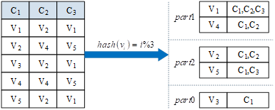
The algorithm is briefly explained as follows. Line 1 initializes \(value2attr\), representing an array of multiple inverted-indexed table sub-tables of size number of threads \(|K|\), where the structure of each inverted-indexed sub-table is a mapping of type String to collection type. Then enumerate each row of each table in turn (lines 2-3), and for each row, enumerate each attribute (line 4), get the value \(value\) of the current record at the current attribute (line 5), and the number of the sub-table \(partNo\) that it should be assigned to under the function \(h\) mapping (line 6), and use the thread numbered \(partNo\) to add that mapping to its sub-table (line 7). The module ends up with the inverted-indexed subtable.
The process is formally expressed as, on database instance \(d\), \({\rm {\mathcal D}}(d)=({\rm {\mathcal U}},{\rm {\mathcal V}},{\rm {\mathcal B}})\), where \({\rm {\mathcal U}}\) denotes the set of attributes, \({\rm {\mathcal V}}\) denotes the set of fetches, binary relation \({\rm {\mathcal B}}\subseteq {\rm {\mathcal V}}\times {\rm {\mathcal U}}\) denotes the set of binary relations from fetches to attributes, the number of threads is \(k\), the hash function is \(h\), and \(S\left(v_{i} \right)\) is defined to be the set of all attribute columns in which \(v_{i}\) is located, then: \[\label{GrindEQ__1_}\tag{1} S\left(v_{i} \right)=\left\{u_{i} |\left(v_{i} ,u_{i} \right)\in {\rm {\mathcal B}},u_{i} \in U\right\} .\] Define the entire inverted index table on \(d\) to be \(I(V,U)\), then: \[\label{GrindEQ__2_}\tag{2} I(V,U)=\left\{\left(v_{i} ,S\left(v_{i} \right)\right)|v_{i} \in V\right\}.\] From the given hash function \(h\), define a subset \(V_{j} ,j\in [1,k]\) of the set of values taken, then: \[\label{GrindEQ__3_}\tag{3} V_{j} =\left\{v_{i} |h\left(v_{i} \right)=j,v_{i} \in V\right\}.\] It is known at this point: \[\label{GrindEQ__4_}\tag{4} \begin{array}{c} {V_{i} \cap V_{j} =\phi ,\forall i,j\in [1,k],} \\ {\bigcup _{i}V_{i} =V,i\in [1,k],} \end{array}\] where \(J\) corresponds to a split-table inverted index table defined as \(I_{j} \left(V_{j} ,U\right)\), then: \[\label{GrindEQ__5_}\tag{5} I_{j} \left(V_{j} ,U\right)=\left\{\left(v_{i} ,S\left(v_{i} \right)\right)|v_{i} \in V_{j} \right\} .\] Eventually there is: \[\label{GrindEQ__6_}\tag{6} I_{i} \left(V_{i} ,U\right)\cap I_{j} \left(V_{j} ,U\right)=\phi ,\forall i,j\in [1,k],\] \[\label{GrindEQ__7_}\tag{7} \bigcup _{i}I_{i} \left(V_{i} ,U\right)=I(V,U),i\in [1,k].\]
At this point it clearly proves the correctness of the method of dividing the inverted index table into multiple smaller tables using the hash function.
General inclusion dependency mining algorithms have either explicitly or implicitly performed a de-duplication (merging) operation on duplicate data values, which has some significance in the practical application of computer algorithms. The values of each column in a data table generally conform to a certain feature or distribution, which results in a portion of the data values being duplicated, and the higher the percentage of duplicated data, the more effective this pruning will be, because this pruning is equivalent to reducing the size of the data from the data unit level.
The example of pruning is shown in Table 1, there are 5 attributes, 5 rows of table, all data values are [1,5], each data is “inverted”, and there are 25 inverted index items in each data, while in attribute column \(A\), there are 5 data in \((1,A)\), and the same is true for other attribute columns, so after pruning the duplicate values, the data volume of 5*5=25 becomes an inverted index item with only 5 entries, and the current efficiency of data value deduplication is \((25-5)/25=80\%\), and only 20% of the data volume needs to be statistically verified.
| A | B | C | D | E |
|---|---|---|---|---|
| 1 | 2 | 3 | 4 | 5 |
| 1 | 2 | 3 | 4 | 5 |
| 1 | 2 | 3 | 4 | 5 |
| 1 | 2 | 3 | 4 | 5 |
| 1 | 2 | 3 | 4 | 5 |
The above example can fully illustrate the superiority of pruning for duplicate values, the following additional example shown in Table 2, the same size of the table, but each attribute contains 1 to 5, that is to say, in the current five attributes, the distribution of its data is the same, the duplicate value pruning can only be merged, to obtain five inverted index entries shaped like \((1,\{ A,B,C,D,E\} )\), and in subsequent mining algorithms, for the “1, 2, 3, 4, 5” are no difference, its same distribution is redundant information, that is, duplicate value pruning can not recognize the duplicate data distribution. And intuitive observation obviously leads to the conclusion that all five attributes are identical and there is interdependence, and this quick response also originates from the observation of attribute data distribution. Therefore, this paper considers the addition of pruning for repetitive data distributions.
| A | B | C | D | E |
|---|---|---|---|---|
| 1 | 1 | 1 | 1 | 1 |
| 2 | 2 | 2 | 2 | 2 |
| 3 | 3 | 3 | 3 | 3 |
| 4 | 4 | 4 | 4 | 4 |
| 5 | 5 | 5 | 5 | 5 |
Repeated-value pruning in the data structure optimizes the overall data structure repetition, but when the data structure repetition rate in the table is not very high, and a large number of different data appear in the same column family, the effect of this pruning is not obvious, especially in the repetition rate is not very high, but in line with the containment dependency of the table, a lot of repetitive inverted index entries many times to carry out statistical validation of a large amount of wasted time and space.
While the distribution of repetitive pruning can be optimized for the distribution of the data structure, the more similar or even the same distribution of the data structure, then the distribution of repetitive pruning effect is better. Intuitively, different data appearing in the same column family are only calculated once.
In Table 1 of the previous section, there is only one data distribution in the 5*5 table, each attribute value field is [1, 5], so the distribution of all the values of its inverted index table is \(\{ A,B,C,D,E\}\), while there are 5 different data values (1 to 5). In fact, after constructing the inverted index table, enumerating the inverted index table no longer requires data values, so the 5 different data values result in redundant distribution values. Pruning the distribution values just solves this problem. Based on the repetitive pruning of the data structure, \((5-1)/5=80\%\) more data are de-emphasized, and only the remaining 20% of the proportion of different distribution values need to be verified. Therefore, after the combined data duplicity and distribution duplicity pruning of the inverted index table, the data value and distribution value of the inverted index table are unique, that is, constituting a “bijection”, the overall de-emphasis efficiency in Table 2 reaches \({\rm (25-1)/25=96\% }\), which greatly improves the linearity of the data structure, and enhances the efficiency of the computer algorithms.
Unlike repetitive pruning of data structures, repetitive pruning of distributions introduces the additional cost of de-weighting the combinatorial cases of all column families, thus gaining the benefit of not having to deal with repetitive combinatorial cases of column families. However, in extreme cases, such as large tables (the number of rows and columns are relatively large) in which almost no data appear in the same column family, the number of combination cases of all column families is \(2^{|U|} -1\), where \(|U|\) is the number of attribute columns, the time and space cost of de-duplication of such a large number of combination cases is exponential.
In this paper, before designing the implementation of GaBP parallel algorithm for the optimization of the linearity of the data structure, it is assumed that the corresponding left end matrix of the linear equations is of order \(n\), and the half bandwidth is \(d\). The bandwidth is \(2d+1\) (the reason for this is that the banded matrices are symmetric). Setting the left end matrix \(A\) of the system of linear equations in a sparse matrix storage method in a column-first manner with a diagonal structure, i.e., \(A_{ij}\) is denoted by \(A[k][j]\), and with \(A[k][j]\), where \(k=1,\cdots ,(2d+1),j=1,\cdots ,n\), there is: \[\label{GrindEQ__8_}\tag{8} i=j-d-1+k.\] In addition, then set up the buffer area between the head and the tail: \[\begin{aligned} \label{GrindEQ__9_} &j=1,\cdots ,d\notag\\ \text{and}\;\;& j=(d+n+1),\cdots ,(2d+n),k=1,\cdots ,(2d+1). \end{aligned}\tag{9}\]
Then the total data storage area has: \[\label{GrindEQ__10_}\tag{10} j=1,\cdots ,(d+n+d),k=1,\cdots ,(2d+1) .\] Therefore, the data storage structure is defined separately for \(A,b,x,x0,p,u,sp,su\) as follows: \[\label{GrindEQ__11_}\tag{11} A[2d+1][m],P[2d+1][m],U[2d+1][m],\] \(m=2d+n\). Then: \[\label{GrindEQ__12_}\tag{12} b[m],x[m],x0[m],sp[m],su[m] .\] The same \(m=2d+n\). Then: \[\begin{aligned} \label{GrindEQ__13_} A_{ij} ,P_{ij} ,U_{ij} ,&j=1,\cdots ,(2d+n),\notag\\&k=1,\cdots ,(2d+1),\notag\\&i=j-d-1+k . \end{aligned}\tag{13}\]
Thus given a \(P[k][j]\) of \(k,j\) corresponding to a \(P_{ij}\), there is: \[\label{GrindEQ__14_}\tag{14} i=j-d-1+k,k=1,\cdots ,(2d+1),j=(d+1),\cdots ,(d+n) .\] Then the \(P_{ji}\) corresponding to \(P_{ij}\) is denoted: \[\label{GrindEQ__15_}\tag{15} P[2d+2-k][j-d-1+k] .\]
That is, if there is \(P_{ij}\) denoted as \(P[k][j]\), then the corresponding \(P_{ji}\) is denoted as: \[\label{GrindEQ__16_}\tag{16} P[2d+2-k][j-d-1+k] .\] With the above representation, the formulas for data structure propagation and updating in the algorithm can be written as the following formulas respectively: \[\begin{aligned} \label{GrindEQ__17_} P\left[k\right]\left[j\right]=&-A\left[k\right]\left[j\right]*A\left[k\right]\left[j\right]/(sp[j-d-1+k]\notag\\ &-P[2d+2-k][j-d-1+k]) . \end{aligned}\tag{17}\]
\[\begin{aligned} \label{GrindEQ__18_} U[k][j]=&-A[k][j]*(su[j-d-1+k]-U[2d+2-k] \notag\\ &[j-d-1+k])(sp[j-d-1+k]-P[2d+2\notag\\ &-k][j-d-1+k]). \end{aligned}\tag{18}\] The steps of GaBP parallel concise algorithm based on data structure linearity optimization include initialization, start of iteration, message accumulation, message updating, solution vector, convergence determination, convergence jump out of iteration, output result and message exchange between nodes. Special treatment is also required for the first computational data node \((q=0)\) and the last node \((q=p-1)\). The first node does not exchange data for its preceding node, and the last node does not exchange data for its following node.
Also for further computer parallel algorithm optimization, the following optimization strategies are used in this paper.
Synchronous GaBP algorithm is used between nodes, while asynchronous GaBP algorithm is used within nodes, so that adding the message accumulation calculation in asynchronous way can accelerate the iteration convergence speed.
For iterative convergence judgment, the judgment can be changed from each iterative step to a strategy of judging after several iterative steps, which reduces the computation required for convergence judgment.
Through the implementation of the above optimization strategy, it can save the data structure exchange space in the operation of computer algorithms, and make the data structure exchange more intuitive and simple, and improve the linearity of the data structure and the algorithmic performance.
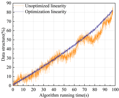
In this paper, in order to explore the change of the linearity of the data structure in the computer algorithm after the improvement using the linearity optimization strategy, the parallel algorithm without improving the linearity of the data structure and the parallel algorithm designed in this paper are compared and analyzed, and the data structure in the operation of the parallel algorithm extracted by mining is taken as an object of analysis, and the linearity of the data structure is analyzed. The results of the analysis of the linearity of the data structure in the computer algorithm are shown in Figure 2, in the parallel algorithm running without optimizing the linearity of the data structure, the computer algorithm running time is less than 45s, and the linearity of the data structure is better, but the slope is too small, and the ability of fast response is insufficient. The running time to 50-70s, the local linearity is better, but the slope is too small, the data structure inflection point occurs, and the response is insufficient in load regulation. 80-100s, the linearity of the data structure is better, but the slope is too large, and the fast response capability is too large. In contrast, in the running time of the algorithm of this study, the linearity of the data structure is better and the slope is reasonable, and there is no data structure change inflection point. This shows that this paper can support the stable operation of the computer algorithm and improve its computational performance by improving the linearity of the data structure.
In this section, seven space truss systems of different scales are used as computational models to verify the correctness, effectiveness and computational scale of the parallel algorithm designed in this paper.Some operations of RDD can be specified by the parameter numTasks to specify the number of tasks for the parallel operation, which are set to the number of RDD’s Partitions as suggested by Spark’s help document, i.e., each Partition is executed by One task for each partition.
For the same computational model, the number of RDD Partitions affects the computational efficiency, in order to maximize the memory computation, Model 4 (DOFs of 2999999) is used as the object to test the computation time under different numbers of Partitions. The Spark platform in this paper has 5 workers, assuming that their performance is the same, and the number of partitions is a multiple of 5 to save the most time, the test results of the parallel algorithm designed in this paper are shown in Table 3 for the computation time under different models and different numbers of partitions.When the number of partitions is less than 30, the memory is overflowed, and the computation is not possible.When the number of parts is greater than 30, the computation time varies with the number of parts. Greater than 30, the computation time increases with the increase of Partition number. Therefore, for the Spark platform in this paper, when calculating Model 4, the best calculation performance can be obtained when the number of Partitions is 30, which can maximize the use of data structure memory calculation. The later calculations are based on this, and the Partition number is adjusted according to the size of the model. As the model size increases, the computation time of the algorithm continues to increase, and the growth rate is getting bigger and bigger, when the model size is larger than 5,000,000 degrees of freedom, the growth of the computation time is more obvious, and the computation efficiency is obviously reduced, and the computation time in 15,000,000 degrees of freedom has reached 22.57h, this is due to the number of computational tasks at this time, the Spark platform is in an oversaturated state, the computational resources competition is large, and the additional computation of the data structure memory can be maximized. The competition for computational resources is large, and the extra overhead of computation is large. Comprehensively, the algorithm in this paper reduces the complexity in large-scale data computation due to the optimization of the linearity of the data structure.
| Calculation time of each model | |||||||
| Models | Model 1 | Model 2 | Model 3 | Model 4 | Model 5 | Model 6 | Model 7 |
| DOFs | 144559 | 485263 | 2100006 | 2999999 | 7999995 | 12000154 | 15000000 |
| Times (s) | 28.4 | 159.6 | 2156.3 | 3567.4 | 26514.3 | 51178.3 | 81263.5 |
| Calculation time of different partition Numbers (Model 4) | |||||||
| Partition | 10 | 20 | 25 | 30 | 35 | 40 | 45 |
| Times (s) | Out Of Memory Error | 3756.9 | 4058.5 | 4256.3 | 4357.4 | ||
In this paper, the Minisat algorithm is selected as the benchmark algorithm for the comparison of experimental results, and its solution speed is far ahead of some other efficient SAT solvers, and it is considered to be the most concise and efficient DPLL algorithm so far. The improved algorithm in this paper solves some difficult stochastic SAT problems by optimizing the linearity of the data structure, and the solving effect is remarkable. After testing the test cases, the algorithm solving results of this paper will be compared with the running results of the Minisat algorithm, which has the best performance so far, for linearity analysis. The hardware environment is a PC with Intel Core2 Dual Core CPU 2.0GHz and 1G RAM. The operating system used is Microsoft Windows XP. The algorithm running platform is Microsoft Visual C++ 6.0.
The test cases in this paper are all harder instances of stochastic 3-SAT problems, which are benchmark problems in SATLIB, and these problems are difficult to solve with general algorithms, so these instances are selected for testing in this paper to show the performance advantages of the parallel algorithms designed in this paper. Some of these instances are satisfiable and some are not, with the number of variables ranging from 100 to 300 and the number of clauses ranging from 500 to 1100. In this paper, 34 sets of hard randomized 3-SAT instances are selected from them. The randomized 3-SAT problem is a very difficult class of SAT problems, which is a big challenge both for the completion algorithms and for the local search algorithms, so it is significant to be able to solve algorithms for instances in this region.
Set the Minisat algorithm’s timeout to 1000s, beyond which the solution will not continue. The running time here refers to the CPU time, and the time unit is second. In this paper, the number of iterations of the parallel algorithm is 100, the number of flips is 10000, the noise parameter is set to 5/10, and the timeout time is 1000s.
In order to better measure the average performance and stability of the algorithm, each group of instances are run 20 times and the average value is taken as the final result. The running results for the satisfiable instances are shown in Table 4. For the satisfiable SAT instances, the solution speed of this paper’s parallel algorithm is improved for almost all instances (except instance uf150-01.cnf). Especially for instances uf175-01.cnf (0.063s), uf225-013.cnf (0.065s), uf225-022.cnf (0.092s), uf250-087.cnf (0.099s), and uf250-089.cnf (0.065s), the speed of the solving is significantly improved. And Minisat’s solution speed even reaches 33.540s when solving the uf225-022.cnf instance, and because this paper optimizes the linearity of the data structure of the parallel algorithm, so that the approximate solution provided by the data structure accelerates the searching process of this paper’s algorithm, and this paper’s parallel algorithm will preferentially search for the subspace in which the approximate solution is located, which ensures that the vast majority of the search process clauses are satisfiable during the search process, thus accelerating the search speed. Therefore, the parallel algorithm designed in this paper is suitable for solving this kind of problems.
| Test case | Variable number | Clause number | The mission at (s) | This algorithm runs time (s) | Whether it can be met |
|---|---|---|---|---|---|
| uf125-01.cnf | 125 | 638 | 0.152 | 0.079 | SAT |
| uf150-01.cnf | 150 | 745 | 0.023 | 0.076 | SAT |
| uf175-01.cnf | 175 | 853 | 6.598 | 0.063 | SAT |
| uf200-01.cnf | 200 | 875 | 0.133 | 0.072 | SAT |
| uf200-021.cnf | 200 | 875 | 0.061 | 0.090 | SAT |
| uf225-01.cnf | 225 | 985 | 0.059 | 0.076 | SAT |
| uf225-013.cnf | 225 | 985 | 8.567 | 0.065 | SAT |
| uf250-01.cnf | 250 | 1087 | 0.038 | 0.068 | SAT |
| uf250-096.cnf | 250 | 1087 | 0.065 | 0.043 | SAT |
| uf225-022.cnf | 225 | 985 | 33.540 | 0.092 | SAT |
| uf225-023.cnf | 225 | 985 | 0.148 | 0.070 | SAT |
| uf225-024.cnf | 225 | 985 | 0.059 | 0.067 | SAT |
| uf225-025.cnf | 225 | 985 | 0.116 | 0.017 | SAT |
| uf250-087.cnf | 250 | 1087 | 11.564 | 0.099 | SAT |
| uf250-088.cnf | 250 | 1087 | 0.144 | 0.016 | SAT |
| uf250-089.cnf | 250 | 1087 | 18.471 | 0.065 | SAT |
| uf250-094.cnf | 250 | 1087 | 0.056 | 0.014 | SAT |
The running results of unsatisfiable instances are shown in Table 5. For the unsatisfiable SAT instances, the solution speed of this paper’s parallel algorithm is slower than that of Minisat’s algorithm, and the average solution time of this paper’s parallel algorithm is 16.677 s, while the average solution time of Minisat’s algorithm is only 11.941 s. When a given formula is unsatisfiable, within the given number of iterations and flip-flops, this paper’s parallel algorithm can not obtain the solution of the original problem. This will inevitably consume part of the solution time. However, the solution speed of this paper’s parallel algorithm is improved by 117.17% compared with Minisat’s algorithm in solving the unsatisfiable SAT instance of uuf250-092.cnf.
| Test case | Variable number | Clause number | The mission at (s) | This algorithm runs time (s) | Whether it can be met |
|---|---|---|---|---|---|
| uuf225-022.cnf | 225 | 985 | 2.562 | 13.365 | UNSAT |
| uuf225-023.cnf | 225 | 985 | 8.794 | 17.222 | UNSAT |
| uuf225-024.cnf | 225 | 985 | 16.552 | 19.248 | UNSAT |
| uuf225-025.cnf | 225 | 985 | 3.265 | 14.783 | UNSAT |
| uuf250-092.cnf | 250 | 1087 | 27.181 | 12.516 | UNSAT |
| uuf250-093.cnf | 250 | 1087 | 11.477 | 14.842 | UNSAT |
| uuf250-094.cnf | 250 | 1087 | 18.417 | 18.483 | UNSAT |
| uuf250-095.cnf | 250 | 1087 | 8.974 | 9.344 | UNSAT |
| uuf250-096.cnf | 250 | 1087 | 19.51 | 26.034 | UNSAT |
| uuf175-01.cnf | 175 | 853 | 25.003 | 29.55 | UNSAT |
| uuf200-01.cnf | 200 | 875 | 5.849 | 11.35 | UNSAT |
| uuf200-09.cnf | 200 | 875 | 13.233 | 16.059 | UNSAT |
| uuf225-01.cnf | 225 | 985 | 10.603 | 16.927 | UNSAT |
| uuf225-06.cnf | 225 | 985 | 5.781 | 18.105 | UNSAT |
| uuf250-01.cnf | 250 | 1087 | 10.175 | 16.498 | UNSAT |
| uuf250-010.cnf | 250 | 1087 | 3.366 | 11.426 | UNSAT |
| uuf250-023.cnf | 250 | 1087 | 12.252 | 17.757 | UNSAT |
Comprehensive analysis of the results shows that the parallel algorithm for optimizing the linearity of the data structure in this paper is not suitable for solving unsatisfiable stochastic 3-SAT problems, but it is more efficient for solving satisfiable stochastic 3-SAT problems. It is suitable for solving satisfiable stochastic 3-SAT problems.
This paper uses multi-threading technology and data pruning method to optimize the linearity of the data structure and design computer parallel algorithm. The linear degree of the optimized data structure and the application effect of the designed parallel algorithm are analyzed, and it is found that:
In the operation of the algorithm without optimized processing of the linearity of the data structure, when the algorithm running time reaches 50-70s, the linearity of the data structure appears to have too small a slope, and at the same time, there is an inflection point of the data structure, which indicates that the algorithm does not have a sufficient response when the load is regulated. And the linearity optimization strategy proposed in this paper has obvious improvement on the linearity of the data structure, the overall linearity is smooth and the slope is reasonable, and the linearity is better.
The parallel algorithm in this paper shows high computational efficiency in dealing with large-scale numerical values, when calculating Model 4, the best computational performance can be obtained when the number of Partition is 30, and the running time is only 3756.9 s. When the model size is 15000000 degrees of freedom, the computational time reaches 81,263.5 s, which is a more obvious growth, but still maintains a high performance.
This paper’s algorithm in the SAT problem solving empirical analysis compared with the most concise and efficient Minisat algorithm, this paper’s parallel algorithm in the solving of satisfiable linear SAT instances solving speed is much higher than the Minisat algorithm. When solving uf225-022.cnf instance, the solution time of this paper’s algorithm and Minisat algorithm is 0.092s and 33.540s respectively, while the solution speed is poorer in solving nonlinear unsatisfiable instances.
Comprehensively, the data structure linearity optimization strategy proposed in this paper can effectively improve the linearity of the data structure in the operation of the algorithm, reduce the time complexity and space complexity of the data structure, so as to enhance the computational efficiency of the algorithm and save the overhead of the computer operation.