Automation technology is growing in popularity as science and technology advance continuously today, and mobile sorting robots are also being developed bit by bit. Applying vision and two-dimensional code technology to the sorting of express mail can significantly increase its efficiency while lowering labour intensity and fostering the growth of the automation sector [1-4]. The four-step method of sorting involves forming a picking action, walking or handling, classification, and picking information [5]. Manual sorting, mechanical sorting, semi-automated sorting, and automatic sorting are common sorting techniques. Automatic sorting, in contrast, can be continuous, high-volume work, lower error rate, and the fundamental realisation of unmanned [6,7], which is becoming increasingly important to the logistics centre.
Robots can now modify their operating object and tools at will, responding to changes in their surroundings thanks to advancements in machine vision and artificial intelligence [8]. When sorting an express in the courier industry, it is not enough to distinguish it based only on its colour and shape; instead, the two-dimensional code on the express must be recognised. Robotic intelligent sorting has gained popularity in the logistics industry as a way to improve sorting accuracy and efficiency. Conventional sorting techniques are frequently limited by the size, shape, and material of objects. However, intelligent logistics sorting robots that utilise machine vision can effectively sort a variety of workpieces by overcoming these limitations with the use of visual perception technology. The goal of this project is to increase the adaptability and flexibility of industrial robots that sort objects in complex environments by equipping them with cameras and utilising machine vision technology to perform autonomous identification, localization, grasping, sorting, and other crucial controls [9].
This paper investigates the use of machine vision techniques for object localization and motion ranging in order to address the challenge of automatically sorting cylindrical workpieces. We have successfully realised monocular motion vision ranging and localization by using point-by-point sampling computation within the robot trajectory in conjunction with the vision library (OpenCV for Python) to process the image data [10]. The experimental results show that the method can achieve the required accuracy under certain conditions, with an average positioning error of less than 4%. This finding has broad application potential and offers dependable technical support for the real-world use of intelligent logistics sorting robots.
The current state and challenges of robot application in the field of logistics sorting will be briefly discussed in this paper, which will be followed by a thorough examination of the machine vision-based control system of an intelligent logistics sorting robot, which includes the essential technologies of autonomous identification, localization, grasping, and sorting. The study’s experimental design and methodology, as well as an analysis and discussion of the findings, are then covered. In conclusion, we provide an overview of the study’s key findings and speculate about potential future research paths in the area of intelligent logistics sorting robot control.
The arm and the end-effector are the two components that make up the manipulator. Figures 1 and 2 display the arm and end-effector’s 3D modelling.
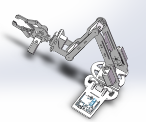

Starting from the bottom of the arm, servos 1 through 5 control the arm’s movement on the Z-axis, servos 2 and 3 control the arm’s positioning to the fastener’s centre in the working platform, servo 4 controls the end-effector’s rising and lowering, and servo 5 controls the hand claw’s attitude. This gives the robotic arm five degrees of freedom. The screw’s lead should be as large as possible to accommodate the rapidity of rising and lowering; the design lead is 2 cm, and the stroke is 8 cm. 3D printing is used to manufacture and assemble the end-effector’s component parts. The end-effector fixture has a clamping torque of 1 N-m and is pneumatic [11].
Three main components make up the mobile sorting robot system: the hardware, software, and mechanical structure. The robotic arm, end-effector, and other components make up the majority of the mechanical structure. The primary controller, camera, servo, LCD screen, air pump, air claw, motor drive, wireless communication module, upper computer, and so on make up the hardware. The self-developed image processing, visual positioning algorithm, and control programme make up the software. The robotic arm control programme and self-developed image processing and visual positioning algorithms make up the software. Figure 3 displays the 3D modelling diagram for the planned mobile sorting robot system.

The robotic arm is represented by 1 in Figure 3, the end-effector by 2, the working area by 3, the camera by 4, and the main controller by 5. The working object of the system is a number of express pieces that have been labelled with QR codes. Each express piece has a QR code that covers specific information about it, and at the express piece stacking point, there is a QR code label that corresponds to the information on each express piece. The robot’s job is to locate the QR code on the express piece and then move it to the appropriate position at the express piece stacking point.
The working area of the system is the field of view captured by the fixed, elevated camera. A number of express mail boxes are arranged at random throughout the workspace. The camera processes the gathered image data to determine the image coordinates of each express mail box’s centre while also identifying the information found on each box’s two-dimensional code label. The robotic arm is positioned to the centre of each express mail directly above using the inferred image coordinates to the robotic arm servo control angle transformation algorithm, allowing the task of grasping and sorting to be finished [12].
As seen in Figure 4, the triangular similarity principle is the fundamental idea behind dimensional measurement of an object using a monocular camera.

The vertical line in Figure 1 between the middle shooting plane and the imaging plane represents the camera’s main optical axis; the symbol \(d\) represents the distance between the lens and the shooting plane; the symbol \(f\) stands for the camera lens’s focal length; the actual measured length of the photographed line segment is represented by \(L\); and the imaged length on the imaging plane (photoreceptor) is represented by \({L'}\). Using the comparable triangle formula, we can obtain:
\[\label{eq1} \frac{f}{d} = \frac{{L'}}{L}.\tag{1}\]
According to the small hole imaging principle, a rectangular region in reality and a pixel of the camera are proportionate to one another, assuming that the camera is not distorted or has an assembly error. The calibration process of the camera, which requires the definition of four coordinate systems, includes the image pixel coordinate system \({C_p}\), the physical coordinate system \(C\) of the image, the camera coordinate system \({C_c}\), as well as the global coordinate system \({C_w}\)—is the solution to the correspondence. The pixel coordinate system and the physical coordinate system of the image can be transformed using the following methods:
\[\label{eq2} \left[\begin{array}{c} x_{\mathrm{p}} \\ y_{\mathrm{p}} \\ 1 \end{array}\right]=\left[\begin{array}{ccc} \frac{1}{\mathrm{~d} x} & 0 & x_0 \\ 0 & \frac{1}{\mathrm{~d} y} & y_0 \\ 0 & 0 & 1 \end{array}\right]\left[\begin{array}{l} x \\ y \\ 1 \end{array}\right],\tag{2}\] where each pixel’s physical dimensions on the \(x-\) and \(y-\)axes are, respectively,\({{\text{d}}x}\) and \({{\text{d}}y}\). The camera coordinate system (\({x_c}\),\({y_c}\),\({z_c}\)) considers the \(x-\) and \(y-\)axes of the image’s physical coordinate system to be the origin \({o_c}\) for the camera’s optical centre and the \({z_c}\) axis for the optical axis. The specific transformation relations are as follows.
\[\label{eq3} z_{\mathrm{c}}\left[\begin{array}{c} x \\ y \\ 1 \end{array}\right]=\left[\begin{array}{cccc} f & 0 & 0 & 0 \\ 0 & f & 0 & 0 \\ 0 & 0 & 1 & 0 \end{array}\right]\left[\begin{array}{c} x_{\mathrm{c}} \\ y_{\mathrm{c}} \\ z_{\mathrm{c}} \\ 1 \end{array}\right].\tag{3}\]
Developed to explain camera position, the world coordinate system (\({x_w}\),\({y_w}\),\({z_w}\)) can also be applied to describe how objects are positioned in the actual world. The translation matrix \(T\) and rotation vector \(R\) of the camera’s outer parameters, which are as follows, can be used to convey how the world coordinate system and the camera coordinate system relate to one another []:
\[\label{eq4} \left[\begin{array}{c} x_{\mathrm{c}} \\ y_{\mathrm{c}} \\ z_{\mathrm{c}} \\ 1 \end{array}\right]=\left[\begin{array}{cc} \mathbf{R} & \mathbf{T} \\ \mathbf{0}^{\mathrm{T}} & \mathbf{1} \end{array}\right]\left[\begin{array}{c} x_{\mathrm{w}} \\ y_{\mathrm{w}} \\ z_{\mathrm{w}} \\ 1 \end{array}\right].\tag{4}\]
Up until now, combining Eqs has provided the relationship between the world coordinate system and the image pixel coordinate system. From Eqs (1) to (4), we have
\[\begin{aligned} \label{eq5} z_{\mathrm{c}}\left[\begin{array}{c} x_{\mathrm{p}} \\ y_{\mathrm{p}} \\ 1 \end{array}\right]=&\left[\begin{array}{ccc} \frac{1}{\mathrm{~d} x} & 0 & x_0 \\ 0 & \frac{1}{\mathrm{~d} y} & y_0 \\ 0 & 0 & 1 \end{array}\right]\left[\begin{array}{llll} f & 0 & 0 & 0 \\ 0 & f & 0 & 0 \\ 0 & 0 & 1 & 0 \end{array}\right]\notag\\ &\times\left[\begin{array}{cc} \mathbf{R} & \mathbf{T} \\ \mathbf{0}^{\mathrm{T}} & 1 \end{array}\right]\left[\begin{array}{c} x_{\mathrm{w}} \\ y_{\mathrm{w}} \\ z_{\mathrm{w}} \\ 1 \end{array}\right]. \end{aligned}\tag{5}\]
When \({z_c}\) is known, monocular ranging can be used to establish the conversion relationship between world coordinates and image coordinates using a calibrated object. On the other hand, when the focal length of the camera is known, it becomes impossible to solve for the depth information of the object in the picture [14].
The binocular camera is a depth camera that resembles the structure of a human eye. It operates on the basis of binocular parallax, with the left and right cameras positioned in the same plane. As illustrated in Figure 5, the imaging parallax is used to calculate the relative distance between the binocular camera and the observation point in the world coordinate system.

The photocentric distance, also referred to as the baseline \(b\), is the distance measured between the projected centres of the two cameras in Figure 2, which shows that two cameras of the same model are positioned parallel to one another. Assuming that the two cameras’ imaging planes are on the same plane, the projected points on the imaging planes of the target \(P({x_c},{z_c})\), which is a point in the scene, are \(P_l({x_l},{y_l})\) and \(P_r({x_r},{y_r})\), respectively.
The similar triangles principle is used to illustrate this once the camera’s focal length, \(f\), is known:
\[\label{eq6} \frac{{{z_{\text{c}}}}}{f} = \frac{y}{{{y_1}}} = \frac{y}{{{y_{\text{r}}}}} = \frac{x}{{{x_1}}} = \frac{{x – b}}{{{x_{\text{r}}}}}.\tag{6}\]
We can get the formula for solving \({x_c}\),\({y_c}\) and \({z_c}\) from the Eq. (7):
\[\label{eq7} \left\{\begin{array}{l} z_{\mathrm{c}}=\frac{f \cdot b}{x_1-x_{\mathrm{r}}} ,\\ x_{\mathrm{c}}=\frac{z_{\mathrm{c}} \cdot x_1}{f}=b+\frac{z_{\mathrm{c}} \cdot x_{\mathrm{r}}}{f} ,\\ y_{\mathrm{c}}=\frac{z_{\mathrm{c}} \cdot y_1}{f}=\frac{z_{\mathrm{c}} \cdot y_{\mathrm{r}}}{f}. \end{array}\right.\tag{7}\]
The depth \(z\) and the parallax value are inversely correlated, according to Eq. (7). When the distance increases, the parallax value decreases. As the distance increases, the parallax value decreases. It is known from the displacement difference \(x\) that the higher the camera pixel, the more accurate the horizontal displacement difference \(x\) can be obtained at the same distance, and the higher the ranging accuracy. We need to know the parallax, \({x_1} – {x_{\text{r}}}\) to solve for the depth \(z\) at a position \(P\), one needs to know the focal length \(f\) of the camera and the distance \(b\) between the left and right cameras. After determining the depth, one can determine \(x\) and \(y\), and then one can determine point \(P\)’s spatial location [15].
Even though binocular cameras have superior characteristics than monocular cameras, direct image prediction and depth estimation from monocular cameras is also a hotspot for application due to advancements in deep learning and image processing algorithms. It is evident from the above binocular ranging principle that positioning and ranging are accomplished by both binocular and monocular vision through the use of the triangular similarity principle. In some circumstances, binocular vision technology can be thought of as a monocular camera that creates parallax by taking pictures at various spatial locations in order to solve depth information. This paper presents a motion vision system that manipulates an industrial camera in a specific way, takes multiple pictures of the same object at different points in the world coordinate system, and uses pixel-matching to extract parallax, which can be utilised to solve the object’s depth information [17]. The schematic diagram of the camera that is being shot at different locations is shown in Figure 6.

The industrial camera is mounted on the end joint of the industrial robot to follow the trajectory, which is a linear motion in the horizontal plane. The focal length of the camera is denoted by \(f\), and the point in the world coordinate system is represented by \({P_{\text{w}}}\) in Figure 6.
The baseline distance formed is the distance in the world coordinate system between the sampling point and the previous sampling point \({b_n} = \sqrt {{{\left( {{x_n} – {x_{n – 1}}} \right)}^2} + {{\left( {{y_n} – {y_{n – 1}}} \right)}^2}}\). The camera records \({P_{\text{w}}}\) points for every distance travelled. The imaging coordinates of the four points at various locations in the figure are \({p_1},{p_2},{p_3},{p_4}\). Figure 6b illustrates how the camera records points \(P\) and \(P'\) while moving from left to right, allowing for the generation of multiple parallaxes \({d_1},{d_2},…,{d_n}\) [18,19].
\[\label{eq8} \left\{\begin{array}{c} d_1=\left|x_{11}\right|-\left|x_{\mathrm{r} 1}\right| \\ d_1^{\prime}=\left|x_{11}^{\prime}\right|-\left|x_{\mathrm{r} 1}^{\prime}\right| \\ d_1=\left|x_{12}\right|-\left|x_{\mathrm{r} 2}\right| \\ d_2^{\prime}=\left|x_{12}^{\prime}\right|-\left|x_{\mathrm{r} 2}^{\prime}\right| \\ \vdots \\ d_n=\left|x_{1 n}\right|-\left|x_{\mathrm{r} n}\right| \\ d_n^{\prime}=\left|x_{1 \mathrm{n}}^{\prime}\right|-\left|x_{\mathrm{rn}}^{\prime}\right| \end{array}\right.\tag{8}\]
Eq. (8) is modified by substituting the average of all parallaxes to get:
\[\label{eq9} \left\{\begin{array}{l} z_{\mathrm{c}}=\frac{f \cdot b}{d_m} \\ z_{\mathrm{c}}\left[\begin{array}{c} x_{\mathrm{p}} \\ y_{\mathrm{p}} \\ 1 \end{array}\right]=\left[\begin{array}{ccc} \frac{1}{\mathrm{~d} x} & 0 & x_0 \\ 0 & \frac{1}{\mathrm{~d} y} & y_0 \\ 0 & 0 & 1 \end{array}\right]\left[\begin{array}{cccc} f & 0 & 0 & 0 \\ 0 & f & 0 & 0 \\ 0 & 0 & 1 & 0 \end{array}\right]\\ \qquad\qquad\qquad\qquad\qquad\times\left[\begin{array}{cc} \mathbf{R} & \mathbf{T} \\ 0^{\mathrm{T}} & 1 \end{array}\right]\left[\begin{array}{c} x_{\mathrm{w}} \\ y_{\mathrm{w}} \\ z_{\mathrm{w}} \\ 1 \end{array}\right] \end{array}\right.\tag{9}\]
The working platform is divided into four areas, and only one express can be placed in each area in order to simplify the visual algorithm processing. The camera uses the four areas to classify the data it collects, making the process easier and more effective. After turning on the system, the camera begins gathering data, and the controller begins binarism of the image data [20,21]. Four expresses with QR codes are positioned at random throughout the allocated area. Apply for 8 cache space, which is used to store the \(X\) and \(Y\) coordinates of the four express white pixel points, respectively. Since the F4 controller can only read memory at a slow speed and can only cache up to three regions at once, the image is processed twice in its entirety. Subsequently, retrieve the middlemost pixel’s \(X\) and \(Y\) coordinates for every region, and transfer the information to the host computer for visualisation. The actual location of the express is displayed in Figure 7 which has a resolution of \(480*480\). The range of \(X\) and \(Y\) is therefore from 0 to 480. Table 1 displays the location information for the express’s centre point.

| (\({x_1},{y_1}\)) | (\({x_2},{y_2}\)) | (\({x_3},{y_3}\)) | (\({x_4},{y_4}\)) |
|---|---|---|---|
| (145,90) | (320,110) | (95,366) | (390,350) |
| (150,90) | (325,120) | (90,366) | (395,355) |
| (156,90) | (318,120) | (98,366) | (389,356) |
| (148,92) | (320,120) | (105,368) | (388,355) |
| (154,90) | (322,120) | (98,357) | (394,355) |
Once each piece’s visual positioning coordinates are known, the robotic arm’s end can be precisely positioned just above the centre of each piece using a transformation algorithm that maps the derived visual positioning coordinates to the robotic arm servo’s angle control pulses [22,23].
The robotic arm places itself exactly above the centre of each shipment, grasps and carries the shipments, sorts the shipments to the designated shipment stacking point, and completes the experimental task based on the information on the identified 2D code label on each shipment. Figure 8 illustrates how the robotic arm’s end grips and handles objects. Following positioning to the target point in Figure 8a, the hand claw’s end lowers; after catching the shipment in Figure 8b, the hand claw rises; in Figure 8c, the robotic arm carries the shipment to the target position; and in Figure 8d, the hand claw is released.

OpenCV offers three common matching algorithms, BM, SGBM, and GC, to solve the parallax maps at various positions after the camera has been calibrated [5]. The camera moves 100 mm to measure a workpiece with a diameter of 60 mm and a height of 10 mm under one condition, as shown in Figure 9, which also includes the parallax depth map and the on-site photographic map. Table 2 displays some of the experimental measurement data. These three algorithms will be chosen for testing in the experiments.
.

| Actual distance/mm | Calculate distance/mm | Relative error/% | Measurement diameter/mm | Calculate diameter/mm | Relative error/% |
| 100 | 90.55 | 9.45 | 60 | 58.65 | 2.25 |
| 110 | 98.48 | 10.45 | 60 | 57.49 | 4.21 |
| 120 | 113.66 | 5.28 | 60 | 58.48 | 2.56 |
| 130 | 122.55 | 5.52 | 60 | 57.85 | 3.56 |
| 140 | 122.84 | 5.52 | 60 | 59.23 | 1.52 |
| 150 | 153.22 | 1.66 | 60 | 60.58 | 1.85 |
| 160 | 163.89 | 2.45 | 60 | 57.86 | 4.23 |
| 170 | 187.52 | 5.21 | 60 | 58.25 | 2.89 |
| 180 | 188.31 | 5.12 | 60 | 58.21 | 2.99 |
| 190 | 198.45 | 4.85 | 60 | 59.87 | 0.45 |
The analysis of the experimental data reveals that, when shooting under varying object distances, the camera will impact the calculation of size and depth; however, within a certain range, it can achieve similar binocular ranging function. The experimental error can be influenced by various factors, including light intensity, background texture and colour, and parallax matching algorithm. Subsequent engineering applications aim to determine the optimal parameters and algorithms in various environments. For example, in the experimental environment, where object distances range from 140 to 160 mm, more precise ranging and positioning error is achieved.
The industry typically uses a fixed camera for image processing to increase the working flexibility of industrial robots. However, this paper creatively installs a monocular camera on the robot joints for motion stereo ranging, further increasing the processing flexibility of the robot. The monocular camera is moved in order to perform the experiment, and to some extent, the binocular camera ranging function can be realised. Fast workpiece positioning and grasping can be achieved in production applications by scheduling the camera’s mobile ranging trajectory to fall inside the workpiece grasping trajectory. This monocular vision ranging technique has a high practical application value in the production line where the accuracy requirement is not strict, and it lowers the cost and difficulty of developing the robot vision system.
There is no specific funding to support this research.