
In the big data era, design is gradually moving towards a new kind of intelligence. The use of algorithms to help designers complete time-consuming repetitive design tasks is one of the main tenets of the current generation of intelligent design research. This study initially uses the three-primary concept to create a set of vector functions in order to precisely measure error distances and create a partitioning model for visual communication. Second, in order to obtain the parameters for visual communication, the scientific encoding of the coefficient constraint features is accomplished, and the relevant hyper-plane is found by carefully extracting the feature information associated to the graphic image. In the end, the BCE With Logits technique can substantially improve the visual communication image represen-tation. The experimental results show that the modified BCE With Logits visual communication design model can be applied to four different types of images with different levels of tedium, and that when the weight parameter is set to 0.34, the accuracy of image recognition rises to 89.59\%, resulting in suc-cessful visual communication.
Design plays a critical role in human society. As a result of the continued development of the Internet, Internet of Things, big data, artificial intelligence, and other technologies, design is increasingly shifting to a new sort of intelligence that is digital, networked, intelligent, and individualised [1,2]. The use of algorithms to help designers complete time-consuming repetitive design tasks is one of the main tenets of the current generation of intelligent design research. The creation of graphic images, which range from ubiquitous posters to web advertisements of all sizes on the internet, shows how the need for various affordable and consumable visual communication designs has always been a challenge [3]. In light of this, research on intelligent image design based on machine learning algorithms has drawn more attention, and the findings are increasingly being used in real-world applications. By learning from a significant amount of accumulated data and material and interacting with simple commands, the Sensei intelligent design tool created by Adobe, for instance, may make repetitive picture alteration simple and automated [4]. The input image can then be transformed into a range of artistic styles. Additionally, a growing amount of research is seeking to tackle more difficult design jobs, such product and archi-tectural design. While algorithms may effectively learn the design principles inherent in the data and batch the design jobs for graphic images, current intelligent design methods are not yet very novel . This not only drastically lowers the bar for design and saves businesses a tonne of money on labour costs, but it also relieves designers of tedious design work and gives them more room for creativity [5,6].
With the advent of data as a component in the visual identity design framework, new media and technologies have also given visual identity design a fresh perspective [7]. The addition of data enables the interpretation of the rich semantics of visual images in addition to their original perceptual repre-sentation, while the sheer volume of data and the visual system’s dynamic nature test the visual system’s ability to be updated and iterated, leading to the development of a new paradigm in computer graphic image technology in addition to the linear static design process [8].
The advancement of intelligent visual identity design will speed up as the usage of dynamic design in visual identity design spreads and the number of media used in visual identity design increases. In order to assist designers in gathering and analysing data and producing designs, the current artificial intel-ligence in intelligent visual identity design is still in the exploratory stage [9,10]. The artificial intelligence technology can be complemented by the design algorithm rules of a designer-led visual identity design system, which can also enhance the thoroughness and completeness of the data collection and analysis stage [11]; moreover, with its iterability and other characteristics, it can not only have a unique visual system for the brand itself, but also adapt to the pace of constant evolution in the age of artificial in-telligence [12].
Visual communication design incorporating parametric logic algorithms will be more logical, scientific, and rigorous in the design process in this context, where the widespread use of parametric computer graphics design has infused new life into the design field and also brought a new perspective to the art aesthetics [13]. Finding a technique to swiftly enable people to accept the information and understand the meaning communicated by the information is a pressing challenge that has to be solved as the in-formation age progresses and the network of complex information data transmits a lot of redundant information to people [14]. To increase their brand awareness and competitiveness in the marketplace, brands are continually updating their visual identities in response to the need for increasingly diversified visual aesthetics. Due to its flexibility and interaction, visual communication pieces created using parametric design can quickly grab the audience’s attention and effectively and without causing them to resist, communicate a brand’s message. Parametric design’s adaptable and colourful visual expression can also accurately convey the brand’s image and tone [15]. The information that is most likely to hold an audience’s attention in a network environment of information overload is that which can be promptly sent to them. In the field of visual communication design, this is particularly relevant for brand visual image design. Science and technology should be used as a constant driving force for the optimisation and development of visual communication design, and visual communication design should work to improve its competitiveness in the network environment of explosive information growth. Visual communication design should also research and analyse the laws governing design development in the context of new media [16].
In conclusion, research on the parametric design of computer algorithms in visual communication design is crucial. The components of visual communication design are affected in a variety of ways by computer graphics technology.
A difficult but useful research subject is the automatic development of graphic layouts, which can aid in both the reduction of highly repetitious typographic work for designers and the intelligent generation of graphic posters by novice users [17]. Numerous real-world situations, like conference posters, trip commercials, magazine covers, etc., might benefit from intelligent visual layout [18]. This study splits the method of intelligent graphic designing into two stages based on this: development of potential graphic layouts based on visual saliency, and rating of potential graphic layouts based on visual as-sessment [19]. The main introduction is candidate graphic layout generation, where the goal of this stage is to generate some potentially harmonious text layouts on natural images given a natural image \({M_i}\) and a piece of text \({T_i}\) , a series of candidate text boxes are output \(M{\text{oset}} = \left\{ {{M_{o1}},{M_{o2}}…,{M_{ok}}} \right\}\) , which differ in the position \({T_p}\) and size \({T_s}\) of these text boxes.
The model proposed in this paper accepts natural images in bitmap form as input and does not require finely annotated visual communication design data, in contrast to some previous approaches to visual communication design layout, which typically require raw fine-grained data, such as categories of images and attributes of design elements [20]. There are two key parts to the development of prospective graphic layouts based on visual saliency.
Visual saliency detection network: The input to this network is the natural image Mi and the output is the corresponding visual saliency map SM.
Text region suggestion algorithm: This algorithm consists of 2 sub-algorithms. The first is the diffusion equation, which uses the text position probability map PDM as an output and the visual saliency map SM as an input. The PDM text location probability map serves as the input for the second algorithm, candidate area generation and the output is a set of candidate text regions with different locations and sizes \(M{\text{oset}} = \left\{ {{M_{o1}},{M_{o2}}…,{M_{ok}}} \right\}\) . Its visual saliency detection network mechanism is shown in Figure 1.
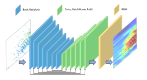
On this basis, we define that the goal of the original BAS Net model is to detect and segment salient objects, but the goal of this section is to compute a visual saliency map at the pixel level, i.e., the saliency value of each pixel is within the real number range of \(\left[ {0,1} \right]\), so the loss function for training is defined as a hybrid loss function, as in Eq. (1).
\[\label{e1} L\left( \Theta \right) = {L_{BCE}}\left( \Theta \right) + {L_{SSIM}}\left( \Theta \right),\tag{1}\] where \({L_{BCE}}\left( \Theta \right)\) denotes the BCE With Logits loss function, \({L_{SSIM}}\left( \Theta \right)\)denotes the \(SSIM\) loss function, and \(\Theta\) denotes the parameters of the visual saliency detection network. Given a real visual saliency map \(G{M_P} \in \left[ {0,1} \right]\) , where \(P = 1,…,N\) represents each pixel and the BCE With Logits loss function is defined as in Eq. (2).
\[\begin{aligned} \label{e2} {L_{BCE}}\left( \Theta \right) = \frac{1}{N}\sum\limits_{p = 1}^N \left( {G_{{M_P}}}\log {S_M}_{_P} + \left( {1 – {G_{{M_P}}}} \right)\right. \times\left.\log \left( {1 – {S_{{M_P}}}} \right) \right), \end{aligned}\tag{2}\] where \({{S_M}_{_P}}\) denotes the visual saliency map of the network prediction.
In this visual communication design model, assuming that \(X = \left\{ {{x_p}|p = 1,2,…,N} \right\}\) and \(Y = \left\{ {{y_p}|p = 1,2,…,N} \right\}\) denote the two image regions extracted from the salient maps \({G_{{M_P}}}\) and \({S_{{M_P}}}\) respectively, \({u_x},{u_y}\) and \(\sigma _x^2,\sigma _y^2\) denotes the mean and variance of \(x\) and \(y\)respectively, and \({\sigma _{xy}}\) is their covariance, the SSIM loss function can be defined as Eq. (3):
\[\label{e3} {L_S}\left( \Theta \right) = 1 – \frac{{\left( {2{\mu _x} + {\mu _y} + {C_1}} \right)\left( {2{\sigma _{xy}} + {C_2}} \right)}}{{\left( {\mu _x^2 + \mu _y^2 + {C_1}} \right)\left( {\sigma _x^2 + \sigma _y^2 + {C_2}} \right)}},\tag{3}\] where \({C_1} = {0.01^2},{C_2} = {0.03^2}\) is a constant set for the training of this network.
In a departure from existing work, and guided by the rules of the specified algorithm, this section applies the diffusion equation to the calculation of the text location probability map, which is defined in Eq. (4).
\[\label{e4} \left\{\begin{array}{c} P D_{M+1}=P D_M+\lambda(d X+d Y) \\ d X=c_X \nabla_X\left(P D_M\right), d Y=c_Y \nabla_Y\left(P D_M\right) \end{array}\right.\tag{4}\] where \({\nabla _X}\) and \({\nabla _Y}\) represent the horizontal and vertical gradients of the pixel, respectively, \({c_X}\) and \({c_Y}\) represent the diffusion coefficients in the two directions, respectively.
When there is a significant difference between the original saliency map and the text location probability map, the iteration comes to an end. The diffusion equation’s application to the calculation of the text location likelihood map is shown in detail in Figure 2.

In this model, the evaluation metrics chosen are the metrics commonly used in saliency detection, the number of mutual relationships, root mean square error and \({R_2}\) coefficient, which can evaluate the similarity between the predicted saliency value of the model and the true saliency value of the image in different aspects. The \({S_M}\) is used to denote the visual saliency map predicted by the network and the \({G_M}\) true visual saliency map, where the number of interrelationships \(CC\) is calculated as in Eq. (5).
\[\begin{aligned} \label{e5} C C\left(G_M, S_M\right) =\frac{\frac{1}{N} \sum_{p=1}^N\left(G_{M_p}-\overline{G_M}\right)\left(S_{M_p}-\overline{S_M}\right)}{\sqrt{\frac{1}{N} \sum_{p=1}^N\left(G_{M_p}-\overline{G_M}\right)^2} \sqrt{\frac{1}{N} \sum_{p=1}^N\left(S_{M_p}-\overline{S_M}\right)^2}}, \end{aligned}\tag{5}\] where \({\overline {{G_M}} }\) and \({\overline {{S_M}} }\) denote the mean values of \({{G_M}}\) and \({{S_M}}\) respectively. The interrelationship number \(CC\) is in the range \(\left[ { – 1,1} \right]\), with higher values indicating greater similarity between the two significant graphs.
In conclusion, the BCE With Logits loss function is frequently used for pixel-level semantic seg-mentation tasks. It aids in obtaining precise region segmentation results at the pixel level, but it is missing a measure for the nature of the surrounding parts. Higher weighted element boundaries aid in obtaining distinct element borders on the visual saliency map. In order to maintain the structure of the original image elements, the SSIM loss function performs better after training with a hybrid loss function that uses the BCE With Logits loss function to maintain a smooth gradient for all pixels. Sections 4 and 5 show experimental findings comparing this visual saliency detection model to al-ternative approaches.
In order to accurately confirm the validity and reliability of the visual communication design method, an experimental comparison was used to comprehensively verify the performance of the approach. Fol-lowing thorough specification of the dataset’s specifications in accordance with the produced graphic picture dataset, 36 images that were comparable to four different types of images were selected and set up as follows:
Class A images. It is mainly used for a comprehensive collection of building decoration images.
Class B images. It is mainly used for a comprehensive collection of pet images.
Class C images. It is mainly used for a comprehensive collection of images of everyday household items.
Class D images. It is mainly used for a comprehensive collection of images of nature scenes.
A sample of 10,000 images was obtained by randomly placing the above 4 images (40 images in total) in the 9960 images, which were then used as the data set. A random sampling process was used to extract 2000 images from these datasets. During the precise characterization of the original image features, attention needs to be given to extracting the image scale using subsets and dividing it so that it is divided into blocks of images of radius, with values typically taken as 16. The structure and content is shown in Figure 3.
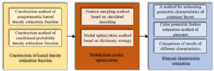
In addition, all feature interval pixel data needs to be set to a uniform 2, where all image scale areas are calculated as \(2R \times 2R\). If the feature distribution fully meets the criteria and requirements of the Gaussian distribution, the fixed scale can be uniformly set to a spatial pyramid scheme, and the program tool used can be configured on a designated personal computer to achieve accurate training of the training samples.
The design features sampled in the dataset are then modeled using a kernel probability density function (as in Eq. (6)), which estimates the distribution patterns of certain design features.
\[\label{e6} K\left( {\frac{{x – x_e^i}}{{{H^{1/2}}}}} \right) = \frac{1}{{{{(2\pi )}^{d/2}}}}\exp \left[ { – \frac{1}{2}{{\left( {x – x_e^i} \right)}^\prime }{H^{ – 1}}\left( {x – x_e^i} \right)} \right].\tag{6}\]
Color design characteristics of different brands of print advertising images can be analyzed by collecting images of different brands of print advertising and then modeling the color features in the images using kernel density estimation. The results of modeling the color features of images related to the keywords “618” and “MUJI” are shown in Figure 4.

In order to determine the effects of parameter changes on other indicators, as shown in Figure 5, it is important to concentrate on testing and analyzing the method’s pertinent parameters in the text, such as the dictionary space capacity parameter of the feature space.

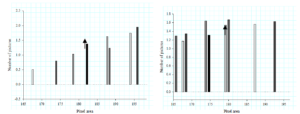
Figure 5 demonstrates how the algorithm’s accuracy tends to climb as the size of the dictionary space does.As the dictionary space becomes closer to 1024 MB, the technique’s accuracy frequently drops, whereas it rises as the number of feature space distributions rises. With 256 MB of feature space distributions, the algorithm’s accuracy is at its highest. It is obvious that the number of feature space distributions and the dictionary space capacity can change significantly, which will have an impact on the accuracy rate of picture recognition. When both parameters are set to 0, the two parameters’ picture recognition accuracy is at its lowest, with corresponding values of 67% and 73%, respectively.
In this scenario, if the distribution of the feature space is set to 256 MB and the dictionary space is 1024 MB, then it is appropriate to do so. In order to effectively balance the image recognition accuracy and recognition efficiency as the image recognition accuracy increases and reaches its maximum value, it is necessary to evaluate and judge the best transmission of the weighting parameters, resulting in the spatially scored image as shown in Figure 6.
Variable mapping relationships between text length and picture encoding configuration parameters were tried, as shown in Table 1, because in this procedure, variable configuration factors of the image encoding may affect the encoding and decoding results. This saves time by eliminating the need to calculate the configuration parameters for the picture encoding dynamically and allowing them to be chosen directly based on the text length Len B each time. The parameter \(\eta\) can be specified by the user, with a larger \(\eta\) indicating that more text information needs to be encoded for each image encoding. By default, \(\eta\) is set to 800.
| Number of text characters | Error correction level | Resolving power |
|---|---|---|
| 1 350 | ’High’ | 100\(\times\)100 |
| 351 1000 | ’Quality’ | 200 \(\times\)200 |
| 1001 2000 | ’Medium’ | 200 \(\times\)200 |
| 2001 2900 | ’Low’ | 300 \(\times\)300 |
It is feasible to effectively use some low brightness colours in addition to text colours with high brightness when the backdrop brightness is in the centre, as shown in Figure 7. When the background brightness is in the middle of the range, it is possible to use both low brightness and high brightness text colours. When using conditional probability estimate approaches rather than kernel density estimation methods, a number of characteristics of the visual design image are more convergent. Additionally, the more convergent results provide the computer more design hints.
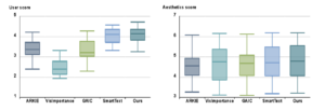
Experiments were done to compare the deep visual scoring model presented in this research with a relevant model from the literature in order to investigate the efficacy of various methods for visually scoring graphic layouts. A general Res Net-based classification model called Smart Text was developed using a dataset of graphic styles with various backgrounds. The fundamental goal of the GIQA model is to estimate the degree of similarity between images from the standpoint of a probability distribution, where the closer an image is to a set of graphic designs with superior visual appeal, the higher its visual score. But neither of these approaches is capable of effectively evaluating the visual quality of various potential text sections on the same backdrop image.
Additionally, as seen in Table 2, the models developed using the AVA dataset had a difficult time differentiating between the candidate text layouts’ visual quality. The fine-grained visual feature-based scoring network’s modules were further studied in the ablation experiments. Because the text regions could only supply a limited number of local image characteristics with distinction, the performance of using solely Ro I features was subpar. In contrast, because Ro E composition characteristics are more discriminative, employing them performs better than using Ro D features. Table 2 supports this chapter’s use of the deep visual scoring model.
| Method | Training data set | IOU | BDE | PCC | SRCC | \(Ac{c_{4/5}}\) | \(Ac{c_{4/10}}\) \(Ac{c_{1/1}}\) | |
|---|---|---|---|---|---|---|---|---|
| Centered layout | – | 0.020 | 0.240 | – | – | – | – | – |
| ARKIE | – | 0.216 | 0.198 | – | – | – | – | – |
| Vis Importance | GDI | 0.209 | 0.204 | – | – | – | – | – |
| GAIC | GAICD | 0.074 | 0.267 | 0.083 | 0.114 | 2.7 | 5.4 | 0.09 |
| TRP+ Res Net (Smax t) | GDI+AVA | 0.107 | 0.260 | 0.004 | 0.006 | 3.55 | 7.6 | 0.10 |
| GDI+TLA | 0.296 | 0.162 | 0.620 | 0.636 | 12.2 | 22.2 | 1.80 | |
| TRP+GIOA | GDI+AVA | 0.098 | 0.262 | 0.004 | 0.005 | 3.2 | 7.3 | 0.10 |
| GDI+TLA | 0.104 | 0.256 | 0.231 | 0.238 | 4.2 | 8.8 | 0.22 | |
| TRP+ Ro I | GDI+TLA | 0.477 | 0.122 | 0.882 | 0.857 | 20.9 | 36.4 | 4.10 |
| TRP+ Ro I + Ro D | GDI+TLA | 0.497 | 0.115 | 0.887 | 0.865 | 27.3 | 43.8 | 4.69 |
| TRP+ Ro I + Ro E | SALICON+TLA | 0.458 | 0.119 | – | – | – | – | – |
| GDI+TLA | 0.530 | 0.310 | 0.889 | 0.868 | 38.5 | 52.7 | 12.29 |
Based on the above optimization effects, the self-encoder-based image information embedding model proposed in this paper can be represented by Figure 8. Firstly, the visual saliency map of the carrier image \({I_c}\) is calculated by the visual saliency network in Section 3 as the visual perception constraint for the subsequent encoding network. Considering the error correction mechanism in information transmission, the textual information \({T_c}\) is converted into the form of image encoding \({I_s}\) input to the encoding network.
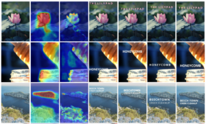
In addition, due to the nature of graphic designs with apparent visual characteristics and clean back-grounds, SteganoGAN models are susceptible to a high decoding error rate. The two methods, Ste-ganoGAN and StegaStamp, are useless for adding information into graphical designs due to these disadvantages, as shown in Figure 9.
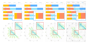
During testing, encoder and decoder can be utilised separately. Due to picture disturbances that are imperceptible to the human eye, the encoded image in Figure 10 is almost identical to the original carrier image. This serves as an example of the outcomes obtained when information is incorporated into a graphic design utilising an encoder network. The residuals between the input carrier picture and the output encoded image were multiplied by ten in order to more clearly show the disturbances brought on by the embedded information. The results show that the encoding network may indirectly embed data while maintaining the aesthetic quality of the original graphic design.

As can be observed, the accuracy of the algorithm grows with the weighting parameter in the shape of a “few” when the dictionary space and the quantity of feature space distributions are 1024 MB and 256 MB, respectively. The image identification accuracy rises to 89.59% when the weighting value is 0.34.
This paper uses three evaluation metrics to calculate the coding quality of the model: peak sig-nal-to-noise ratio, structural similarity, and image perceptual similarity. the PSNR metric is widely used to evaluate the degree of distortion of images and is calculated as in Eq. (7] and Eq. (8].
\[\label{e7} PSNR = 20 \cdot \left( {{{\log }_{10}}{P_{\max }} – {{\log }_{10}}\frac{1}{N}\sum\limits_{p = 1}^N {{{\left( {{I_{{c_p}}} – {I_{{c_p}}}^\prime } \right)}^2}} } \right).\tag{7}\]
\[\label{e8} \operatorname{SSIM} ({\text{x}},{\text{y}}) = \frac{{\left( {2{\mu _x}{\mu _y} + {C_1}} \right)\left( {2{\sigma _{xy}} + {C_2}} \right)}}{{\left( {\mu _x^2 + \mu _y^2 + {C_1}} \right)\left( {\sigma _x^2 + \sigma _y^2 + {C_2}} \right)}}.\tag{8}\]
In this empirical model, set \({C_1} = {0.01^2},{C_2} = {0.03^2}\) , in line with the theoretical model.
For a fair comparison, the carrier images tested were resized to the same size and data of the same size were embedded in the test images and higher \(PSNR\), higher \(SSIM\) and lower \(LPIPS\) indicate better visual results of the encoded images after embedding the information. As shown in Table 3, the comparison results show that the method in this chapter is able to embed information into various types of graphic designs while ensuring better visual quality.
| Method | Image size | 100 bits/P | 100 bits/S | 100 bits/L | 3200 bits/P | 3200 bits/S | 3200 bits/L |
|---|---|---|---|---|---|---|---|
| Steg Stamp | 400 \(\times\) 400 | 34.10 | 0.9313 | 0.0414 | – | – | – |
| Steg an GAN | 400 \(\times\) 400 | 35.27 | 0.9387 | 0.0248 | 35.20 | 0.9381 | 0.0250 |
| This method | 400 \(\times\) 400 | 40.64 | 0.9960 | 0.0008 | 39.20 | 0.9931 | 0.0009 |
| This method | 800\(\times\) 800 | 42.09 | 0.9991 | 0.0004 | 41.71 | 0.9988 | 0.0005 |
By asking viewers to choose the encoded image that differs the least visually from the original carrier image, the comparison experiment also included a user survey to assess the visual impact of encoding using various information steganography algorithms. The survey chose 15 carrier images from the test dataset, produced the encoded images using three different information embedding techniques, and enlisted 30 participants to complete the survey in order to choose the optimum embedding outcome for each carrier image. The poll results showed that the models in this chapter had an average selection rate of 83.6%, while SteganoGAN and StegaStamp had selection rates of 15.1% and 1.3%, respectively. According to the aforementioned experimental findings, the technique used in this chapter produces better visual results in terms of information embedding encoding quality than the other methods, as demonstrated in Figure 11.
The visual quality of the encoded image decreases when more data is embedded, which is one of the difficulties in embedding large amounts of information in a graphic design. Therefore, experiments were conducted to evaluate the visual quality of the encoded images after embedding different lengths of text information using the codec network in this chapter. The resolution of the carrier image used for testing was set at 1600 \(\times\) 1600. Figure 12 shows the results of the evaluation of the visual quality of the encoded visual quality of this chapter’s model, where the axis represents the number of bits of input text and the axis represents the average of the corresponding image quality evaluation metrics. These metrics show that the model is able to ensure good visual perception of the encoded graphic design even when implicitly embedding information on larger data sizes.

As it is difficult to embed larger scale data in a graphical design using the Stega Stamp method, the chapter model was compared with two other methods, LSB and Deep Steg. In this experiment, the test dataset used had a range of image resolutions of \(\left[ {300 \times 300,3000 \times 3000} \right]\) and the performance evaluation table is shown in Table 4.
| Method | Watermark | Brightness | Rotation | JPEG |
|---|---|---|---|---|
| LSB | 0.03% | 0% | 0% | 0% |
| Deep Steg | 3.46% | 32.76% | 100% | 9.9% |
| This method | 55.30% | 32.80% | 100% | 10.3% |
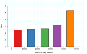
Additionally, tests were carried out to determine how quickly the techniques in this chapter would insert text messages of various lengths in carriers with varying resolutions, and the findings are displayed in Figure 13. Where the Y axis represents the typical processing time (in seconds) for the entire encoding and decoding process, and the X axis represents the quantity of incoming text content. The different colored dashes indicate different resolutions of the carrier image in the range \(\left[ {200 \times 200,1600 \times 1600} \right]\).
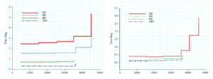
It can be demonstrated that very constant temporal performance can be exhibited throughout the en-coding phase of the visual communication model when embedding text information of varying lengths into a carrier image of the same resolution. The visual saliency map of the carrier picture, the best information embedding region, the creation of a 2D code, the feeding of the matching image region with the 2D code into the encoding network, and finally the acquisition of the encoded image are all steps in the process of fully encoding an image. The 2D code is what takes the most time to create while the image resolution is constant and the amount of text information to be encoded grows, even though the encoding network itself is relatively quick in terms of computing. On the other hand, a significant factor in the variance in time performance for embedding information in carrier images of different resolutions is the computation of the ideal information embedding region and the visual saliency map. The time overhead for decoding images of different resolutions is comparable since the decoding network is so quick. While decoding greater scale data, the recovery of the QR code into text takes longer.
An idea for assembling vector functions for visual communication design components and building a model for partitioning visual communication based on computer graphic image technology. Using this method, picture distortion can be avoided while implicitly including visual communication information into the image.The experimental findings of this study demonstrate that the BCE with Logits correc-tion-based visual communication design model can be applied to four categories of images with varying levels of annoyance. When the weight parameter is set to 0.34, the image recognition accuracy increases to 89.59%, producing a positive visual communication effect.
There is no specific funding to support this research.