he general population like tennis because it is simple to learn and has few field limits in everyday life [1]. The number of people playing different sports is rising, as is the investment in sports consumption, thanks to the successive introduction of national sports consumption policies and the growth of sports. This has greatly aided in the development of intelligent tennis research and development [2,3]. tennis aficionados need a professional coach who can play with them anytime and anywhere and has a high level of skill; this encourages the creation of intelligent tennis robots. The primary issue facing tennis is the shortage of suitable sports opponents [4].
Computer vision, image processing, trajectory planning, full-court localization, motion control, mechanical design, and other technologies are being used to create completely autonomous tennis robots [5,6]. The core of developing fully autonomous tennis robots is computer vision and image processing. These fields require solutions to issues like motion blur, multi-scale, short-time occlusion, background clusters, etc. These issues arise in tennis because it is a small target game, and they must be resolved in order to design a vision system with high accuracy, high real-time, and strong robustness. This system then uses these features to detect and track tennis in real-time, determine the position of the game, predict the tennis ball’s landing point, and ultimately realizes the tennis robot hitting the ball [7].
Target detection and tracking research has been the subject of numerous high-quality publications from domestic and international university laboratories, research institutes, and enterprise teams. These findings have found successful applications in the domains of security, automated driving, and new retailing [8]. For tennis training, real-time is essential since players must respond swiftly and the ball moves quickly. Reducing latency to fulfill real-time needs is a difficulty for current vision systems, which may experience difficulties in real-time, particularly when processing massive amounts of data and images. Since tennis is played in a range of lighting, field, and backdrop circumstances, accurate identification and tracking require a vision system that is resilient to changes in light and interference from the surrounding environment [9,10]. Since tennis is played in a range of lighting, field, and backdrop circumstances, accurate identification and tracking require a vision system that is resilient to changes in light and interference from the surrounding environment. Because tennis balls are small targets with limited physical dimensions, it may be difficult to recognize them in photographs. To address this issue, finer image processing techniques and higher resolution are needed. It can be difficult for the visual system to interpret and filter out background noise when there are a lot of different details and motions in the background of tennis movement [11,12].
Visual enhancement techniques can effectively reduce noise in the image, improve image clarity, and provide more details, which is very important for dealing with complex backgrounds and improving the accuracy of small target detection [13]. They can also improve image quality and make the vision system more capable of accurate detection and tracking in low-light conditions, which is very helpful for indoor or low-light scenarios [14]. By reducing jitter and blurring and increasing image stability, visual improvement techniques can increase tracking and position prediction accuracy. The current vision systems for real-time, accurate, and robust tennis assisted training need to be continuously enhanced. To increase the functionality and performance of tennis robots, additional research and technological innovation will be needed to address the aforementioned difficulties.
YOLO is an extremely quick real-time target detection technique. Fast real-time detection is crucial in tennis assisted training to catch moving tennis balls, and YOLO’s speed advantage makes it the best option [15]. Because tennis balls are very small targets, YOLO’s small-target detection ability aids in the precise recognition and tracking of tennis balls [16]. YOLO works well in this area. When combined, the YOLO model’s outstanding real-time, small-target recognition, and multi-scale processing capabilities make it a potent tool for resolving today’s problems in visual systems for tennis assisted training. When combined with other visual enhancement methods, YOLO can provide more precise tracking, position prediction, and tennis ball detection.
In light of this, this paper improves the related vision algorithms that are currently in use in the 2D image plane to realize the lateral detection, tracking, and trajectory prediction of flying tennis balls in video streams. This is done in response to the vision system’s need to realize these functions.
In this paper, we present a novel detection and tracking algorithm that combines the machine learning algorithm AdaBoost with the conventional three-frame difference technique. This algorithm can accurately identify tennis balls in flight and track their trajectories. This research presents two new tennis detection networks, M-YOLOv2 and YOLOBR, and optimizes the deep learning one-stage detection network Tiny YOLOv2 in order to increase computational efficiency and accuracy. By conducting comprehensive testing and assessment on video streams of flying tennis in four straightforward and intricate scenarios, we show in this study the higher performance of the enhanced tennis identification algorithm and the deep learning network.
Rectangular features, another name for HAAR image feature descriptors, were initially used for target tracking and detection in the face domain of video streams.The primary method used by HAAR to compute image features is the use of feature templates. Common HAAR feature templates fall into four basic categories, which are edge, linear, center, and diagonal features, as illustrated in Figure 1.
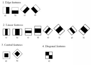
Simple black and white rectangles combined in each direction can realize the extraction of image features, as shown in Figure 1. The categories, sizes, and positions of the feature templates determine the HAAR feature values, which results in a significant increase in the computation of HARR image feature extraction. Because of this, the HAAR integral map emerged later. By going through the entire image once, one can obtain the pixel value of each image position and, at the same time, describe the global feature information of the image, reducing the feature computation time. The schematic diagram of the HAAR integral map is displayed in Figure 2. For any position point \(x\) in the image, the value of the image can be obtained by calculating the Eq. (1).
\[\label{e1} p(x,y) = p(x – 1,y) + p(x,y – 1) – p(x – 1,y – 1) + f(x,y).\tag{1}\] In the integral image, \(p(x,y)\) denotes a pixel value at position \((x,y)\), and \(f(x,y)\) denotes a pixel value at point \((x,y)\) of the original image.
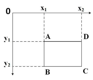
The following Eq. (2) yields the cumulative total of the pixel values in the rectangle ABCD region, as seen in Figure 2:
\[\label{e2} S(ABCD) = S(C) + S(A) – S(B) – S(D),\tag{2}\] where \(S\) is the region of the integration map’s cumulative sum of the pixel values.
Furthermore, target detection and tracking in video streaming are commonly accomplished through the use of HOG and LBP image feature descriptors.By extracting local picture characteristics, HOG has considerable resistance to situations with evident lighting changes, but its real-time performance is low and its effect is poor for images with severe geometric deformation and high speed motion .Target detection in complex situations where the target’s local texture features need to be coupled with the environmental context performs poorly overall because to LBP’s great resistance to picture grayscale and rotation, as well as the target’s well-characterized local texture features lacking global information.Moreover, targets in video streaming are found using LBP. When it comes to target detection in complicated scenarios where the environmental context must be taken into account, LBP performs poorly generally due to its lack of global information and strong robustness to image gray scale, rotation, and local texture properties of the target. After using the integral image for feature value computation, HAAR may significantly cut the feature computation time and increase the algorithm’s real-time performance when compared to HOG and LBP. It can also express the global information of the entire image. In order to obtain a tennis feature model that can be utilized to identify tennis, this study employs the HAAR image feature descriptor to extract tennis image features for the AdaBoost algorithm training.
AdaBoost is a feature-engineered machine learning method in the Boosting algorithm series. To enhance comprehension of its premise, the subsequent concepts (1) and (2) along with Figure 3 are provided.
Optimal weak classifier: It is known from integration learning theory that random guessing performs worse than weak classifiers (in binary choice issues, the error rate must be less than 50%), and this is a significant factor in the integration outcome at the end.
Cascade classifier: given N best weak classifiers \({h_i}\), a cascade classifier H is obtained by weighted linear combination and symbolization of the best weak classifiers \({h_i}\), which is computed as in Eq. (3] and Eq. (4):
\[\label{e3} f(x) = \sum\limits_{i = 1}^N {{\alpha _i}} {h_i}(x).\tag{3}\]
\[\label{e4} H(x) = \operatorname{sign} (f(x)).\tag{4}\]
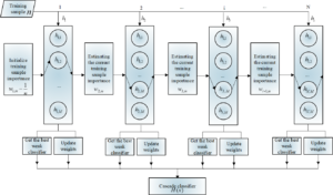
From Figure 4, it can be seen that based on the idea of boosting tree, the AdaBoost algorithm cascades the best weak classifiers \({h_i}\) obtained at each stage of learning in the previous stage, and finally obtains a cascade classifier H .During the learning period, several iterations need to be carried out, and in the first iteration \({T_1}\), each training sample is given the same weight, i.e., \({w_{1,m}} = \frac{1}{n}\) (n indicates the total number of training samples, and m indicates the mth training sample). After the first iteration \({T_1}\) of training, the first best weak classifier 1h is obtained. Thereafter, the weights of the current training samples are updated based on the results of the previous iteration. For the i-th iteration T , if a training sample is correctly classified during the i -1th iteration, its sample weight in T is reduced; on the contrary, if a training sample is misclassified, its sample weight in T is increased. After the training of the i-th iteration \(T\), some sets of weak classifiers with weak features of the training samples are obtained, and feature selection is performed under the threshold rule to obtain the best weak classifier \({h_i}\). The above process is repeated until all the iterations are completed, and finally a cascade classifier \({h_i}(x)\) is obtained by linearly weighted superposition of the best weak classifiers. During the training process, the weights of the training samples are normalized to reduce the effect of illumination.
The corresponding algorithm flow is as follows:
Given the training sample set \(\left( {{x_1},{y_1}} \right),\left( {{x_2},{y_2}} \right), \ldots ,( {{x_i}},\) \({{y_i}}), \ldots ,\left( {{x_N},{y_N}} \right)\), this paper \({x_i}\) represents the video stream in the two-dimensional image plane of the tennis related information, such as: tennis relative to the coordinates of the upper left corner of the whole image, tennis image resolution, etc., \({y_i}\) represents the labeling information, the tennis or background samples.
Set the weights of the training samples to zero for the first iteration: \({w_{1,m}} = \frac{1}{n}\) ; where \({w_{1,m}}\) indicates the weight of the m th training sample, subscript 1 denotes the first iteration, and \(n\) denotes the total number of training samples.
In the i th iteration \((i = 1,2,3,…,N)\), repeat the following operations:
Standardize the input training sample weights:
\[\label{e5} {w_{i,m}} = \frac{{{w_{i,m}}}}{{\sum\limits_{m = 1}^n {{w_{i,m}}} }},\tag{5}\] where \({w_{i,m}}\) denotes the initial weight of the m th training sample during the i-th iteration.
For all training samples, calculate the feature weighted error rate \({\varepsilon _i}\):
\[\label{e6} {\varepsilon _i} = \sum\limits_{m = 1}^n {{w_{i,m}}} \left| {{h_i}\left( {{x_m}} \right) – {y_m}} \right|,\tag{6}\] where h denotes a weak classifier.
The best weak classifier \({h_i}\) with minimum error rate \({\varepsilon _i}\) is obtained:
\[\label{e7} {h_i} = \mathop {\arg \min }\limits_{{h_i}\left( {{x_m}} \right)} \left( {{\varepsilon _1},{\varepsilon _2}, \ldots ,{\varepsilon _n}} \right).\tag{7}\]
Overall sample weights updated: \[\label{e8} {w_{i + 1,m}} = {w_{i,m}}\delta _i^{1 – {e_m}}.\tag{8}\]
\[\label{e9} {\delta _i} = \frac{{{\varepsilon _i}}}{{1 – {\varepsilon _i}}}.\tag{9}\]
Generate a cascade classifier to obtain the tennis feature model:
\[\label{e10} H(x)= \begin{cases}1 & \text { if } \sum_{i=1}^N \alpha_i h_i(x) \geqslant \sum_{i=1}^N \alpha_i \\ 0 & \text { otherwise }\end{cases}\tag{10}\] where, \({\alpha _i} = \log \frac{1}{{{\delta _i}}}\).
A Four-Year Old tennis Detection Algorithm
Deep learning one-stage series of detection algorithm YOLO was developed for this reason. Early target detection algorithms were primarily realized by “manual feature extraction,” “target classification,” and other ideas, which can guarantee the accuracy in specific scenes, but the detection speed is slow, robustness is weak, and labor costs are high. The most recent version of YOLOv3 has a mAP of 57.9% for 80 different sorts of objects (AP50 standard) and a fastest detection speed of 30 frames/sec for photos with a resolution of \(608*608\) by a Titan X on the COCO test set.Yolo has steadily increased the speed and accuracy of its detections, and to a certain degree, it can meet the real-time and accuracy standards for tennis detection. In this section, we improve the YOLO simplified version of network Tiny YOLOv2 in terms of loss function and network structure to improve the tennis ball detection performance (speed and accuracy) in order to obtain more useful tennis ball coordinates for the detection problem that the flying tennis balls in the video stream are small targets.
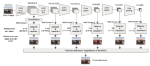
Figure 4 depicts the construction of the YOLOv1 network, which comprises of the initial 24 convolutional layers, the middle 6 maximum pooling layers, and the final 2 fully connected layers. A basic 1×1 reduction layer, which determines the number of convolutional kernel channels for downscaling and upscaling, and a standard 3×3 convolutional layer alternate between the convolutional layers. While the Tiny YOLOv1 network, a condensed version of the YOLOv1, has fewer convolutional layers (9 layers) and can recognize objects more quickly (150 frames/s), it has a low recall and a large error for determining the offset of the border relative to the labeled box. It is a big error.
Eq. (11) illustrates the computational expression for YOLOv1, which use the sum of error squares as the loss function:
\[\label{e11} \begin{aligned} L=&\lambda_{\text {coord }} \sum_{i=0}^{s^5} \sum_{j=0}^B 1_{i j}^{\text {obj }}\left[\left(x_i-\hat{x}_i\right)^2+\left(y_i-\hat{y}_i\right)^2\right] \\ &+ \lambda_{\text {coord }} \sum_{i=0}^{S^2} \sum_{j=0}^B 1_{i j}^{o b j}\left[\left(\sqrt{w_i}-\sqrt{\hat{w}_i}\right)^2+\left(\sqrt{h_i}-\sqrt{\hat{h}_i}\right)^2\right] \\ &+ \sum_{i=0}^{S^2} 1_i^{\text {obj }} \sum_{c \in c \text { casses }}\left(p_i(c)-\hat{p}_i(c)\right)^2. \end{aligned}\tag{11}\]
From Eq. (11), the YOLO loss function consists of three parts: localization error, IOU error, and classification probability error. \({1_{i}^{obj}}\) represents whether the object appears in cell i or not, \({1_{ij}^{obj}}\) represents that the i th bounding box predictor in cell \({1_{ij}^{obj}}\) detects the presence of a target and is responsible for predicting the corresponding target, and \(j\) represents that the th bounding box predictor in cell i detects the absence of the target. \((x,y)\) represents the center coordinates of the bounding box, \((w,h)\) represents the width and height of the bounding box, and c represents the confidence score. \({p_i}(c)\) represents the probability that the object belongs to category i if it appears in cell c . In order to improve the stability of the model during the training process, parameters \({\lambda _{{\text{coord }}}}\) and \({\lambda _{{\text{noobj }}}}\) are introduced, which are applied to weight the predictive loss of the bounding box coordinates and the predictive loss of the confidence without including the object bounding box, respectively \(({\lambda _{{\text{coord }}}} = 5,{\lambda _{{\text{noobj }}}} = 0.5)\).
In 2018, YOLOv3 was offered as a way to significantly increase the target identification accuracy of YOLOv2. While YOLOv3 employs binary cross-entropy loss for both model training and bounding box multi-class prediction, a novel feature extraction network called Darknet-53 is created for the extraction of picture features by leveraging the shortcut connection concept seen in Resnet networks.
Although YOLO can satisfy the requirements for real-time tennis detection, a few issues still need to be fixed.To detect two images, YOLOv1 splits them into \(S*S\) cells, predicts two bounding boxes for each cell, and then determines the probability of C object categories and the object confidence of each bounding box. The model’s capacity to anticipate targets is somewhat constrained by the amount of projected bounding boxes per cell. Small targets, like tennis balls and grouped objects (like birds, ants, etc.), are still difficult to identify, despite the original authors’ proposal of the more effective YOLOv3. This part improves the network structure and loss function of the simpler YOLO network, Tiny YOLOv2, to make it better suited for tennis detection. The resultant modified network is known as YOLOBR.
Tiny YOLOv2 penalizes the localization and classification errors in order to maximize the error sum of squares in the output. By forecasting the square root of the bounding box’s width and height with the same deviation of the boxes, the model locally reflects that small bounding boxes have a bigger impact on the overall detection effect than large ones, as indicated by the YOLO generalized loss function expression (11). But since flying tennis balls in the video stream are considered small targets (with resolutions ranging from \(20*20\) to \(40*40\) pixels), the loss function may be calculated easily by utilizing the anticipated bounding box’s width and height. Furthermore, since there is only one kind of tennis as the target detection object in this paper, the categorization portion of the loss function is deleted, yielding a new loss function expression (12), whose detailed notation is defined in Eq. (12), and which is referred to as “M-YOLOv2” in this part of the network. This reduces the weight of the model and improves the detection efficiency.
\[\begin{aligned} L=\lambda_{\text {coord }} \sum_{i=0}^{S^2} \sum_{j=0}^B 1_{i j}^{\text {obj }}\left[\left(x_i-\hat{x}_i\right)^2+\left(y_i-\hat{y}_i\right)^2\right] +\lambda_{\text {coord }} \sum_{i=0}^{S^2} \sum_{j=0}^B 1_{i j}^{b j j}\left[\left(w_i-\hat{w}_i\right)^2+\left(h_i-\hat{h}_i\right)^2\right] + \sum_{i=0}^{S^2} \sum_{j=0}^B 1_{i j} 1_{j j}\left(C_i-\hat{C}_i\right)^2 +\lambda_{\text {noobj }} \sum_{i=0}^{S^2} \sum_{j=0}^B 1_{i j}^{\text {noobj }}\left(C_i-\hat{C}_i\right)^2. \end{aligned}\tag{12}\]
M-YOLOv2 can somewhat enhance tennis detection when compared to Tiny YOLOv2, but it can still be improved. The semantic properties of tennis images learned in the network structure would be weakened by the frequent use of the pooling layer, which is not good for small object detection. Therefore, as indicated in Table 1, “M-YOLOv2” is improved to produce the new tennis detecting network, YOLOBR.
| Layer Type | Filters | Size/Stride | Output |
|---|---|---|---|
| Input | – | – | 426×426 |
| Convolution | 4 | 1×3/1 | 426×426 |
| Convolution | 4 | 3×1/1 | 426×426 |
| Convolution | 8 | 1×3/1 | 426×426 |
| Convolution | 8 | 3×1/1 | 426×426 |
| Maxpool | – | 4×4/4 | 124×124 |
| Convolution | 16 | 1×3/1 | 124×124 |
| Convolution | 16 | 3×1/1 | 124×124 |
| Convolution | 32 | 1×3/1 | 124×124 |
| Convolution | 32 | 3×1/1 | 124×124 |
| Maxpool | – | 4×4/4 | 28×28 |
| Convolution | 64 | 1×3/1 | 28×28 |
| Convolution | 64 | 3×1/1 | 28×28 |
| Convolution | 128 | 1×3/1 | 28×28 |
| Convolution | 128 | 3×1/1 | 28×28 |
| Maxpool | – | 2×2/2 | 15×15 |
| Convolution | 256 | 3×1/1 | 15×15 |
| Convolution | 256 | 3×1/1 | 15×15 |
| Convolution | 30 | 1×1/1 | 15×15 |
| Convolution | 256 | 3×1/1 | 15×15 |
| Convolution | 256 | 3×1/1 | 15×15 |
| Convolution | 30 | 1×1/1 | 15×15 |
As shown in Table 1, YOLOBR reduces the number of maximal pooling layers from 6 layers in M-YOLOv2 to 3 levels in order to enable the network to gain greater semantic information about small objects. One maximum pooling layer follows every four layers in the first twelve convolutional layers. Research has demonstrated that employing asymmetric decomposition, which involves utilizing one layer of 1×N and one layer of N×1 convolutional layers rather than one layer of N×N convolutional layers, can improve the efficiency of the trained model. YOLOBR employs a similar strategy to improve the overall accuracy of the tennis image by replacing each 3×3 convolutional layer before the maximum pooling layer with a 1×3/1 convolutional layer and a 3×1/1 convolutional layer, with the exception of the final 1 layer of convolutional layer, which uses a regular ReLU activation function. The other layers are added with Leaky ReLU, and the final detection layer uses Softmax to output the results. The nonlinear representation of tennis picture features is enhanced by the network as a whole.
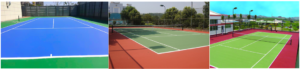
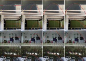
The dataset needs to have a large number of high-quality, diverse, and other conditions in order to meet the training requirements of the deep learning YOLO series detection network and machine learning AdaBoost on tennis sample data. This is done to prevent the model from overfitting and to help the network better learn the features of the data. The tennis dataset must be gathered manually because easily accessible internet datasets as Pascal VOC, COCO, OTB-50, etc. are unsuitable for method validation in this work. To be more precise, the tennis dataset was created from 15 video streams (1280 x 720 pixels) that were laterally recorded by the ZED camera under various conditions. Approximately 18,000 RGB three-channel flying tennis images with a resolution of 1280x720x3 are utilized for testing and training models. Each video stream has an effective duration of approximately 40 seconds and a frame rate of 30 frames per second. The tennis resolution varies from 20×20 to 40×40 pixels, making it a small target. The exterior wall of the engineering hall, which has a variety of colored backgrounds, the laboratory, the parking lot, the woods, the side of the highway, and other locations are among the shooting settings. These scenes are categorized as basic or difficult based on the backgrounds, lighting, and interfering objects.
The outer wall of the engineering hall serves as the primary simple scene in the experimental video, with a single orange, brown, green, etc. serving as the background color. Throughout the video filming, the light and brightness levels were consistent. As seen in Figure 4, there are hardly any moving items other than the tennis ball.
Scenes that are complex include parking lots, forests, and labs. A lot of clutter is present when filming; white walls, cars, sunlight shining through trees that closely resembles the color of tennis, people moving around a lot with rackets, and constantly oscillating tree trunks and leaves produce dramatic variations in light and brightness (Figure 6).

Furthermore, 500 more static photographs of tennis in various settings are gathered in order to enhance the tennis model’s feature expression capability. The dataset is divided into two sets: the training set, which consists of approximately 12,000 images (10 video streams), and the test set, which consists of the remaining 6,000 images (5 video streams of tennis flights on the orange wall, blue wall, green wall, laboratory, and parking lot, respectively). The training set and test set do not overlap.
Targeted preprocessing is needed in order to truly convert the aforementioned acquired dataset into image data that can be used for deep learning YOLO model training and machine learning AdaBoost.
Regarding hardware, this paper’s experiments are all carried out on a Dell mobile image workstation outfitted with an i7 CPU, 16GB of RAM, and an 8GB NVIDIA M1200 graphics card. Software-wise, this section employs Windows 10 as the operating system, the OpenCV3.1.0 computer vision library, the Visual Studio2017 software platform, and C++ programming to perform tennis tracking experiments.
In recent years, the machine learning tracking algorithms AdaBoost and FTOC have been combined with some classical tracking algorithms, such as TLD, MIL, correlation filter series tracking algorithms KCF and Context-aware Discrete Correlation Filter (DCF_CA), and deep learning tracking algorithms Dynamic Siamese Network (DSN) and Co-trained Kernelized Correlation Filter (COKCF), etc. for the purpose of experimental comparison and result analysis. These combinations are based on the combination of the three-frame difference algorithm.
AdaBoost and FTOC design tests to validate the impact of FTOC on tennis ball tracking performance. 1200 frames from a test set of lab tennis flight video streams are chosen by the experiment for testing, and obtains the indexes of recall rate \({r_c}\) , failure rate \({r_m}\) , false positive rate and frame rate \({r_fp}\) . Except for \({r_fp}\) (this shows the proportion of tracked tennis balls by incorrect recognition to total balls in the video stream.
In particular, AdaBoost and FTOC are utilized to perform tennis recognition and tracking, respectively, based on three-frame differencing, median filtering, image binarization, and morphological closure operations on the image to obtain a complete motion foreground.
The detectMultiScale function in OpenCV3.1.0 is used to carry out the “multi-scale” recognition (the image scaling ratio is set to 1.1) and each target is recognized as a tennis at least eight times. The AdaBoost algorithm imports the feature model file cascade.xml to realize the tennis recognition. At least eight times, each target is identified as a tennis ball. To achieve tennis tracking, FTOC integrates the intrinsic features of tennis flight based on three-frame differencing and AdaBoost. The tennis balls in the test video stream have sizes ranging from 20×20 to 40×40 pixels. In Algorithm 1 in Section 3, the values for dmax, Pmin, Pmax, Amin, and Amax are 150, 80, 160, 400, and 1600 pixels, correspondingly. Furthermore, IOU is fixed at 0.5, so that tennis tracking and recognition succeeds when IOU \(>\) 0.5 and fails when IOU \(>\) 0.5. Table 2 displays the outcomes of the experiment.
| Algorithm | $$r_c$$ (%) | $$r_m$$ (%) | $$r_fp$$ (%) | FPS(%) |
| Frame Difference + Adaboost | 78.88 | 21.11 | 2.75 | 10.42 |
| FTOC | 94.51 | 5.44 | 1.50 | 10.69 |
| FTOC without BS | 72.55 | 27.39 | 10.41 | 4.82 |
As shown in Table 2, while maintaining similar computational efficiency FPS with the AdaBoost algorithm incorporating three-frame differencing, the FTOC algorithm has improved the tennis tracking recall rate \({r_c}\) , false positive rate \({r_fp}\) , etc. The recall rate \({r_c}\) is increased from 78.88% to 94.51%, and the false positive rate \({r_p}\) is decreased from 2.75% to 1.50%. The FTOC algorithm is a principle that enhances tennis tracking performance. It operates on the following principles: when tennis detection fails, it activates the “detection-based tracking” mechanism. The FTOC tracking algorithm is initialized using the most recent tennis detection points obtained by the AdaBoost algorithm. It then obtains the tennis and consecutive frames of both internal and external attributes of the tennis in flight, which satisfy the FTOC algorithm’s requirements. Then, using the two consecutive frames with internal and exterior attributes during the flight, the possible positions of Euclidean distance, area, perimeter, etc. between the tennis and those frames are obtained (blue rectangular box in Figure 7). As a result, one-way tennis allows for the acquisition of more tennis points during play, which helps with precise tennis trajectory prediction and subsequent development of the optimal striking strategy.
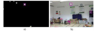
Additionally, it is taken out of “FTOC” and labeled as “FTOC without BS,” i.e., the AdaBoost recognition algorithm, in order to demonstrate the significance of the three-frame difference technique on the tennis tracking efficiency and recall. The experimental findings are displayed in Table 2. Table 2 final row displays the experimental outcomes. A tennis picture search screen is displayed in Figures 8(a) and 8(b) for the “FTOC” and “FTOC without BS” lab settings, respectively. It can be observed that the “FTOC” image processing screen becomes relatively simple after applying the difference algorithm, which increases computational efficiency; however, “FTOC without BS” requires feature matching and target search to be performed across the entire complex image screen without the integration of the three-frame difference algorithm, which could result in tennis error. However, “FTOC without BS” necessitates feature matching and target searching throughout the entire complicated picture frame, making it vulnerable to misidentification in tennis, resulting in a low recall rate (\({r_c}\)= 72.55%), a high false positive rate ( \({r_fp}\)= 10.41%), and a low computational efficiency ( FPS= 4.82 frames/sec).
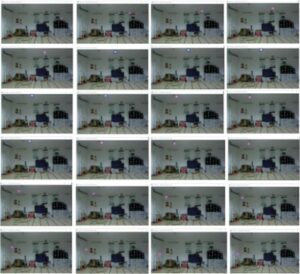
Figure 8 illustrates how the FTOC algorithm affected a portion of the tennis tracking video streams from one-way tennis flights in the lab using 24 randomly chosen images. The pink circle represents the tennis that AdaBoost recognized, the blue rectangle box represents the tennis that the FTOC algorithm tracked using three-frame differencing and AdaBoost additional tracked tennis (in this order: from top to bottom, from left to right), and some tennis (the first row, the first column) could not be identified or tracked. There are certain tennis balls that are neither tracked or identified (row 1, column 1).
Both FTOC and the traditional tracking algorithms that have been used in recent years are used to tennis tracking in order to better examine the performance of FTOC algorithm on tennis tracking. First, a 1200-frame video stream of tennis flight is tested in the lab as part of the tests, and the recall rate \({r_c}\), failure rate \({r_m}\) and frame rate FPS are obtained, and the experimental results are shown in Table 3.
| Algorithm | \({r_c}\) (%) | \({r_m}\) (%) | FPS(%) |
|---|---|---|---|
| FTOC | 94.51 | 5.44 | 10.69 |
| TLD | 18.32 | 81.57 | 6.88 |
| MIL | 52.13 | 47.88 | 11.31 |
| KCF | 29.62 | 70.42 | 46.29 |
| DCF_CA | 76.35 | 23.61 | 19.22 |
| DSN | 85.85 | 14.15 | 6.35 |
| COKCF | 84.29 | 15.69 | 10.89 |
Table 3 demonstrates how poorly TLD and MIL work when tracking tennis, where the game may be tracked in the beginning phase and lost in the rising phase in the top video stream. Table 3 shows that the failure rate rm is greater than or close to the recall rate \({r_c}\). In particular, TLD takes a longer time to update the fern classifier, which leads to lower computational speed (FPS =6.88 frames/sec). MIL is close to FTOC in terms of real-time performance ( FPS=11.31 frames/sec), but has a lower tennis tracking recall (\({r_c}\) =52.13%).
Correlation filtering-based tracking algorithms like KCF, DCF_CA, and SAMF_CA demonstrate their benefits in terms of frames per second. Of them, KCF (46.29 frames/sec) meets the tennis robots’ real-time tracking requirements to a large extent; nevertheless, the tracking recall(\({r_c}\)=29.62%) is low, and the DCF_CA tracking algorithm performs more computationally efficiently ( FPS=19.22 frames/sec). Nevertheless, the correlation filter series-based tracking algorithm is less resistant to background clusters, substantial illumination changes, easy occlusion, and rapid target motion. Although the weight model taught online slows down the deep learning based tracker DSN’s computing performance (6.35 frames/sec), it performs better in terms of recall (85.85%) than the conventional correlation filter tracking algorithm KCF.By applying deep convolutional features, COKCF surpasses the conventional correlation filter KCF tracking algorithm in tennis tracking, as measured by recall (\({r_c}\) =84.29%).The FTOC tracking algorithm works better than the conventional correlation filter KCF tracking method in that it maintains a moderate tracking speed (10.69 frames/sec) and achieves the maximum recall (94.51%) and lowest failure rate (5.44%).
It is known from Chapter 4.2 that another index of tracking techniques is the center localization error, or CLE. Table 3 is used to identify the top three tracking algorithms with the highest recall rate: FTOC, DSN, and COKCF. 1200 frames of tennis flight video streams are used for the CLE calculations and result analyses in the simple scenario’s green wall and the complex scenario’s laboratory, respectively. According to the experiment, tennis tracking succeeds if the CLE is less than 15 pixels (the predefined value), and vice versa. Table 4 displays the experiment outcomes by computing the average CLE of each algorithm.
| Scenery | FTOC | DSN | COKCF |
|---|---|---|---|
| Green Wall | 3.55 | 3.33 | 2.67 |
| Lab | 6.12 | 12.59 | 11..65 |
| Average | 4.87 | 7.92 | 7.16 |
Table 4 shows that the three tracking algorithms have good localization performance when it comes to tracking tennis. The experiments show that the FTOC algorithm has a high localization accuracy for tennis tracking. Of them, the average CLE of FTOC in the simple scene green wall is 3.55, which does not achieve the best result. However, its CLE in the laboratory of complex scene and the average CLE of two scenes reach the lowest (respectively, the average CLE of the laboratory is 6.12 and the average CLE of two scenes combined is 4.87).
This experiment uses the FTOC algorithm for tennis tracking to four different tennis flight video streams (1200 frames per scene), namely the parking lot, the orange wall, the green wall, and the laboratory, to confirm the scene robustness. The FTOC technique is tested ten times for each video stream with the IOU set to 0.5. The average values of the \({r_p}\) ,\({r_c}\), \({F_1}\) metric, and FPS are computed, respectively, and the experimental results are displayed in Table 5.
| Scenery | \({r_p}\) | \({r_c}\) | \({F_1}\) | FPS (Frames/second) |
|---|---|---|---|---|
| Orange Wall | 97.15 | 90.92 | 93.93 | 19.77 |
| Green Wall | 95.11 | 93.68 | 94.38 | 26.31 |
| Laboratory | 90.92 | 89.48 | 90.17 | 7.35 |
| Parking Lot | 92.51 | 69.65 | 79.45 | 7.12 |
| Average | 93.94 | 85.93 | 89.76 | 15.14 |
As shown in Table 5, the FTOC algorithm based on the “tracking by detection” mechanism incorporates some intrinsic properties of the tennis ball itself and the flight process through a simple and effective data-driven technique, and achieves high precision \({r_p}\) (97.15% and 95.11%, respectively), recall (90.92% and 93.68%, respectively), and real-time tracking speed \({r_c}\) (19.77% and 26.31 frames/sec, respectively) for the simple scenarios of an orange wall and a green wall. \(FPS\) (90.92% and 93.68%, respectively) and real-time tracking speed \({r_c}\) (19.77% fps and 26.31 fps, respectively) in simple scenes such as orange wall and green wall. For the complex scenes, especially the parking lot, the image processing efficiency is greatly reduced by light, wind, and more other interferences (FPS is only 7.12 frames/sec), and the background clustering problem is serious, which makes it easy to mis-tracking phenomenon, and thus leads to a lower result of the overall metrics (the integrated 1F metric is only 79.45%). However, the average values of \({r_p}\) ,\({r_c}\), \({F_1}\) metric and for the four scenes are 93.93%, 85.93%, 89.76% and 15.14 fps respectively. Overall, the results demonstrate the better performance of the FTOC tennis tracking algorithm in terms of recall, precision, and real-time performance, along with its great scene resilience.
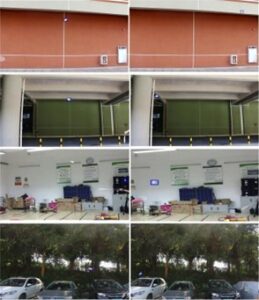
Some of the FTOC’s tennis tracking results are displayed in Figure 9, where the tracked tennis balls are indicated by blue rectangular boxes. Among these, motion blur and background clusters cause certain tennis balls to be mistracked and missed (row 3, column 1).
This section uses a series of detection networks, including Tiny YOLOv2, M-YOLOv2, and YOLOBR to achieve tennis detection. The experimental objects used in this section are video streams of tennis flights (1200 frames per video stream) in both simple and complex scenarios.
This section designs comparative experiments with Tiny YOLOv2, M-YOLOv2, and YOLOBR in order to verify the superiority of YOLOBR network in tennis detection performance. The experimental datasets consist of four video streams of tennis flights (1200 frames per video stream), namely, the orange wall, the green wall, the laboratory, and the parking lot. The input image is compressed from 1280 x 720 to 416 x 416, with an IOU of 0.5 and an NMS of 0.8 (confidence level) during the tennis detection process. Each detection network runs 10 tests for every video stream, and the precision \({r_p}\) , recall ,\({r_c}\), \({F_1}\) metric, and frame rate \(FPS\) are computed. The results of each scene and the scene averages are displayed in Table 6 -Table 10, respectively.
| Algorithm | \({r_p}\) | \({r_c}\) | \({F_1}\) | FPS (Frames/second) |
|---|---|---|---|---|
| Tiny YOLOv2 | 95.5 | 75.8 | 84.3 | 29.8 |
| M-YOLOv2 | 96.0 | 97.8 | 97.1 | 29.6 |
| YOLOB | 98.7 | 97.6 | 98.0 | 30.4 |
| Algorithm | \({r_p}\) | \({r_c}\) | \({F_1}\) | FPS (Frames/second) |
|---|---|---|---|---|
| Tiny YOLOv2 | 90.7 | 89.3 | 90.2 | 28.3 |
| M-YOLOv2 | 95.2 | 98.8 | 97.1 | 28.8 |
| YOLOB | 95.5 | 98.2 | 96.5 | 31.4 |
| Algorithm | \({r_p}\) | \({r_c}\) | \({F_1}\) | FPS (Frames/second) |
|---|---|---|---|---|
| Tiny YOLOv2 | 68.2 | 85.7 | 76.1 | 26.6 |
| M-YOLOv2 | 85.2 | 90.5 | 87.8 | 27.5 |
| YOLOB | 96.2 | 92.5 | 94.6 | 28.8 |
| Algorithm | \({r_p}\) | \({r_c}\) | \({F_1}\) | FPS (Frames/second) |
|---|---|---|---|---|
| Tiny YOLOv2 | 87.5 | 42.8 | 57.5 | 24.6 |
| M-YOLOv2 | 90.2 | 96.5 | 93.2 | 24.7 |
| YOLOB | 96.5 | 94.2 | 95.5 | 26.4 |
| Algorithm | \({r_p}\) | \({r_c}\) | \({F_1}\) | FPS (Frames/second) |
|---|---|---|---|---|
| Tiny YOLOv2 | 85.6 | 73.5 | 78.8 | 27.2 |
| M-YOLOv2 | 91.8 | 96.5 | 93.2 | 27.5 |
| YOLOB | 96.8 | 95.6 | 96.1 | 29.3 |
Table 6–10 demonstrate how, in four scenarios, the combined performance of YOLOBR and M-YOLOv2 enhanced on Tiny YOLOv2 outperforms Tiny YOLOv2, particularly in the laboratory and parking lot where precision and recall are significantly greater. For straightforward situations involving the orange and green walls, M-YOLOv2’s precision and recall are comparable to YOLOBR’s, but they are inferior to YOLOBR’s for more complicated scenarios involving the parking lot and laboratory. In basic settings like orange and green walls, M-YOLOv2’s precision and memory are comparable to YOLOBR’s; but, in complicated scenarios like parking lots and laboratories, M-YOLOv2’s precision and recall are inferior to YOLOBR’s. In comparison to M-YOLOv2’s measurements of the same conditions (97.1%, 87.8%, and 93.2%), YOLOBR’s F1 metrics for the orange wall, laboratory, and parking lot are higher at 98.0%, 94.6%, and 95.5%, respectively. In contrast, M-YOLOv2 (96.1%) has a lower average value of F1 metric than the four scenes’ combined average of 93.2%, which is determined by YOLOBR.
In the dataset of part 5 for tennis trajectory prediction tests, a one-way tennis flight is intercepted in this part from each of the four tennis flight video streams: blue wall, green wall, parking lot, and laboratory. The distribution of tennis frames ranges from 25 to 60, contingent upon the duration of flight. The Euclidean distance between the tennis trajectory prediction point and the labeled point, or the center localization error, is used to quantify the accuracy of the tennis trajectory prediction method.
The FTOC algorithm tracked n tennis coordinate points during the ascending phase of a one-way flight. These points were then used to calculate the trajectory equation, which was fitted using the least-squares method (the quadratic function solves the hyperbolic equation). The trajectory equation was then used to determine the tennis pre-prediction points for the duration of the flight, and the pre-prediction points were optimized using the standard Kalman filtering algorithm.
When the first two to nine tennis coordinate points obtained during the rising phase of the game are used for fitting, the actual tennis flight trend is not well predicted for the four one-way tennis flight video streams; when more than ten points are used for trajectory fitting, the prediction effect is essentially no longer improved. Ten tennis coordinate points are selected for trajectory prediction since the experiment finds that getting as few coordinate points as feasible in the ascending stage improves the prediction effect. A selection of the tennis trajectory prediction outcomes under various fitting points, as determined by the least squares method, are displayed in Figure 10. The black solid circle represents the tennis ball labeling points, the blue solid rectangle represents the tennis ball coordinate points tracked by the FTOC algorithm, and the light blue inverted triangles represent the tennis ball prognosticating points obtained by the least squares method. The red curve represents the curve obtained by the least squares method for the first 10 coordinate points (green solid triangles) obtained in the rising phase of the tennis ball. The outcomes of the least squares method’s trajectory prediction with 2, 3, 10, and the total number of tennis coordinates acquired during the ascending phase of the flying tennis in each scenario are displayed in Figure 10, respectively (see Table 11 for details)
| Scene | Blue Wall | Green Wall | Laboratory | Parking lot |
|---|---|---|---|---|
| Number of tennis coordinates | 12 | 17 | 16 | 13 |
Using 10 tennis coordinate points for trajectory prediction, Figure 11 displays the experimental outcomes. The 2D fitting curves (a) and related 2D CLE distribution curves (b) of various scenarios of the one-way tennis flying process are shown in Figure 11. Black solid circles (tennis labeling points), blue solid squares (tennis coordinate points identified and tracked by the FTOC algorithm), green solid rhombuses (tennis coordinate points predetermined by the least squares algorithm), and red solid triangles (tennis coordinate points optimized by Kalman filtering) are the curves obtained by fitting, respectively, in (a). The red and green curves in (b) are the results of fitting solid circular and triangular points, respectively. These curves represent the 2D CLE distribution curves of the labeled points and tennis coordinate points optimized by Kalman filtering and the predetermined tennis coordinate points and labeled points by the least squares method. The marked values on the curves represent the 2D CLE maximum of the curves, and the appearance of certain breaks in the middle indicates that the FTOC algorithm did not recognize the tracking tennis ball.
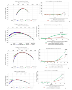
The black and blue curves in the four scenes almost coincide during the one-way tennis flight, as seen in Figure 11. This suggests that the tennis coordinate points obtained by the FTOC algorithm in the corresponding image frames are reasonably accurate; however, Table 11 demonstrates that the number of tennis coordinate points acquired in each scene’s ascending phase varies.The 2D fitting curve (green curve) created by the least squares method is more closely aligned with the actual tennis flight curve (black curve) due to the higher accuracy of the tennis coordinate points gathered during the climbing phase of the simple scenes (blue wall, green wall). Because the tennis coordinate points for the simple scenarios (blue wall, green wall) were more precisely obtained during the rising phase, the two-dimensional fitted curves produced by the least squares method (green curves) had a trend that was more in line with the real tennis ball flight curves (black curves). Furthermore, the red curve indicates that, following Kalman filtering, the optimal tennis coordinate points are nearer the real flight trajectory. The 2D CLE pixel interval of the basic scene is less than that of the complex scene, as Figure 11 illustrates decreased error intervals for [0, 119.94], [0, 190.07], and [35.74], respectively.
In this study, we focus specifically on the tracking, trajectory prediction, and detection of tennis balls in flight. In order to reliably identify and track the motion trajectory of tennis balls, we provide a novel detection and tracking algorithm that combines the conventional three-frame differencing technique with the machine learning algorithm AdaBoost. Furthermore, we offer two new tennis detection networks, M-YOLOv2 and YOLOBR, and optimize the deep learning one-stage detection network, Tiny YOLOv2, to increase computational efficiency and accuracy. These networks perform exceptionally well in terms of real-time tennis detection, recall, and accuracy.
Using video feeds of tennis in flight in four straightforward and intricate scenarios, we thoroughly tested the deep learning networks and the enhanced tennis recognition algorithm in our studies. The experimental findings demonstrate that YOLOBR makes notable gains in average recall, average precision, and average frame rate for tennis identification, with corresponding averages of 95.7%, 96.7%, and 29.2 frames/sec.