ith the development of globalization of the economy, it leads to changes in the organizational scale and production organization of enterprises, which tend to be more project-oriented. Project scheduling problems exist in various industries, especially in the engineering project construction industry, project scheduling has become an efficient and necessary planning and management technology. Traditional research on project scheduling problems has been deepened and refined to form a more scientific theoretical system [1, 2, 3].
For repetitive construction projects like highway and railroad projects, due to its own special construction characteristics. That is, there are relatively few processes, and the construction of some of these processes is continuous and repetitive, or even continuous and repetitive within the entire project. Still using the method will make the original continuous process discrete, so that the time continuity of the project implementation and the continuity of the use of resources can not be guaranteed. The repetitive project scheduling problem that cannot be solved effectively has led to the emergence of many studies on repetitive project scheduling methods [4, 5, 6].
Under the background of big data, a new method of preparing project scheduling plan, the line planning method, has been gradually studied in the field of domestic engineering project scheduling research. The method addresses the execution characteristics of repetitive construction projects and proposes a planning technique suitable for such continuous construction projects. The line planning method is widely used in pipeline laying, highway construction and other projects. Such projects, which are performed continuously and repetitively in spatial locations, are called line projects. Adopting a different representation from network diagrams, the optimization method of using repetitive project schedule plan diagrams to represent the project schedule is called repetitive project scheduling method [7, 8, 9].
Currently, academic theories generally agree that the repetitive project scheduling method technique has more obvious advantages when used for repetitive projects. This is because the construction progress of repetitive projects can be well described in the two-dimensional coordinates of time and spatial location using this technique [10, 11].
Literature [12] proposes a new approach for scheduling repetitive processes. It aims to reduce the probability of missing deadlines while reducing the resource idle time. A discrete simulation approach is used to evaluate the feasible solutions (sequence of cells) from the perspective of scheduling robustness. Literature [13] developed a flexible repetitive scheduling model. And verified the practicality and effectiveness of the model with greater flexibility in minimizing the project duration and cost. A future direction may be to combine the current model with more realistic setups or other scheduling optimization problems. Literature [14] developed a GIS location-based plan for a highway project constructed in a hilly area in order to demonstrate the capabilities of GIS. The study concluded that GIS can be used as a stand-alone system for developing integrated location-based plans for highway construction projects in hilly terrain. Literature [] proposed a multi-objective project scheduling model for simultaneous optimization of time, cost, quality, resource usage and disruption time. The effectiveness and superiority of the model in MRPSP-PSCC is verified through an example study. Literature [16] proposed a multi-objective optimization model considering time, cost, resources, environmental impact, safety and quality based on a newly developed multi-objective optimization algorithm (NSDE-R). The TOPSIS algorithm is combined with the optimization algorithm. A construction project is taken as an example to verify the applicability of the model. A mixed-integer linear programming model for the scheduling problem is given in literature [17]. The objective is to schedule a portfolio of projects in a way that minimizes the total cost, indirect cost, and delay penalties associated with resource idle time can be solved by a general-purpose solver. The model is applied to the portfolio scheduling of multi-family residential projects. Literature [18] proposes a deterministic approach to coordinate the work in the project to construct multiple buildings with a repetitive process in inhomogeneous units. A particle swarm algorithm is used for optimization and demonstrated by a project to construct duplex dwellings.
This paper clarifies the workflow of LOB scheduling method for repetitive projects, divides the types of repetitive project processes based on the influence of control processes on the total duration of repetitive projects, and analyzes the calculation of time parameters of LOB scheduling method. Combined with the description of resource-constrained project scheduling problem, put forward the conditional assumptions of resource-constrained repetitive project scheduling optimization model, establish the objective function as well as the constraints of LOB resource allocation, solve the optimization of LOB resource allocation by using the branching limit algorithm, and make clear the step-by-step process of LOB scheduling resource optimization allocation algorithm based on the branching limit algorithm. Analyze the performance of different LOB scheduling methods, use construction project examples for LOB scheduling duration problem description, and perform LOB scheduling resource allocation for construction scheme duration optimization.
The repetitive project scheduling problem is mostly found in engineering construction projects such as buildings and bridges. Its distinctive feature is that each project can be subdivided into a number of process systems, and each process system has more than one similar process. For example, in the construction of multi-storey buildings, the project can be subdivided into multiple floors of the construction, each floor of the building process is similar, can be used as a process system. Another example is the multi-storey building “wall painting” process, can be divided into “painting the first layer”, “painting the second layer”, etc., each layer is an indispensable process of the entire project.
Repetitive construction projects are generally categorized into two types, vertical repetitive construction projects and horizontal repetitive construction projects. The former type such as high-rise building construction, housing projects. The latter, such as bridge projects, pipeline projects, railroad projects and so on. To solve the general project scheduling problem Dozmo uses the network planning diagram to find control routes, compressed schedule, etc. are very convenient, but for this project scheduling problem has many shortcomings.
Since repetitive projects are extremely common in engineering, and often have large investment and long lead time, many researches on scheduling methods for repetitive projects have emerged.
The Line of Balance (LOB) method is a recurring project scheduling method that utilizes a two-dimensional graphical tool for schedule control and planning of recurring projects.
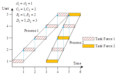
In the LOB diagram, the horizontal axis represents time, the vertical axis represents units, and each inclined bar represents a process, with no overlap between processes, and each process consists of the same number of units. Each process can be constructed by several task forces at the same time, and the rotation between task forces is shown in Figure 1.
Take the project in the figure as an example, the project contains 2 processes, each process contains 5 units, the unit duration of process 1 and process 2 are 1 day, the total duration of process 1 is 5 days, and the total duration of process 2 is 3 days. Process 1 is constructed by one team alone, with a productivity of 1 (team/day), and is constructed one by one according to the order of the units. Process 2 is a multi-team construction situation, the production rate of 2 (team / day), team 1 on the first unit of construction is completed, the third unit of construction, and then the fifth unit of construction. Similarly, team 2 is required to work on the second and fourth units.
Once the control route for a recurring project has been identified, the processes that are on the control route can be identified as control processes. According to the impact of the control process on the total duration of the repetitive project, the control process is divided into three categories, positive control process, reverse control process and point control process.
Positive control processes, i.e., if the extension of the duration of the control process will lead to the extension of the total duration, then such processes are defined as positive control processes.
The conditions for determining a positive control process are:
The process is located on the control route.
The productivity of the process is less than that of its immediate preceding and following processes. If there is no immediate preceding or following process, i.e., the process is located at the beginning or end of the position, then this process is also a positive control process.
Inverse control process, i.e., if the extension of the duration of the control process will result in the shortening of the total duration of the project, such process is defined as an inverse control process.
Inverse control process is determined by the condition that the process is located on the control route and the productivity of the process is greater than its immediate preceding and following processes.
Point control process, i.e., point control process is defined as a process in which there is one and only one unit located on the control route. This unit is connected to the first or last unit of its immediate preceding and following processes. If the realization of this control point is delayed, the total project duration will be delayed, otherwise it is not affected.
A point control process is determined if the process is located on the control route and the productivity of the process is greater than that of either its immediate preceding or immediately succeeding process.
In order to ensure continuity in the construction of the process and to minimize the idle time of the teams, the productivity of the process should be related to the number of teams employed as follows: \[\label{GrindEQ__1_}\tag{1} R_{i} =\frac{C_{i} }{d_{i} } ,\] \[\label{GrindEQ__2_}\tag{2} D_{i} =d_{i} +\frac{N-1}{R_{i} } .\]
In the above equation, \(C_{i} =\) process \(i\) number of task forces, \(d_{1} =\) process \(i\) duration of a unit, \(R_{i} =\) process \(i\) productivity, \(N=\) number of units in the process, \(D_{i} =\) process \(i\) duration.
LOB method time parameter calculation is divided into two parts, one is the time parameter calculation of the internal unit of the process, and the other part is the time parameter calculation between the processes. First of all, the calculation of time parameters of the internal unit of the process is introduced, assuming that the start time of the \(j\)nd unit of the process \(i\) is \(S_{in}\) and the end time is \(F_{ij}\), and the start time of the process is specified to be \(S_{i1} =0\), and the start time of the two units neighboring each other is different from the start time of the unit \({1\mathord{\left/ {\vphantom {1 R}} \right. } R}\), then there are: \[\label{GrindEQ__3_}\tag{3} \begin{array}{c} {S_{i1} =0F_{i1} =S_{i1} +D_{i} } ,\\ {S_{i2} =S_{i1} +1/R_{i} F_{i2} =S_{t2} +D_{i} } \\ {\cdots }, \\ {S_{ij} =S_{i(j-1)} +1/R_{i} F_{ij} =S_{ij} +D_{i} }. \end{array}\]
Obviously, the start time and end time of each unit of the process are in an equidistant series, and by iterative induction of the above formulae, then the start time and end time of the \(j\) unit of the \(i\) process can be expressed in the following form: \[\label{GrindEQ__4_}\tag{4} S_{\imath } =\frac{j-1}{R_{i} } {\rm \; \; }F_{\imath } =\frac{j-1}{R_{t} } +D_{i} .\]
For the calculation of time parameters between processes, the first step is to determine the logical relationship between processes. When two neighboring processes are SS type, i.e., the productivity of a process is higher than the productivity of the process immediately after it, the SS type relationship between processes is shown in Figure 2. Then the start time and end time of the latter process are: \[\label{GrindEQ__5_}\tag{5} S_{1+1} =S_{1} +d_{1} {\rm \; \; }F_{l+1} =S_{t+1} +D_{1} .\]
When two adjacent processes are of FF type, i.e., the productivity of a process is lower than the productivity of the process immediately after it, and the FF-type relationship between processes is shown in Figure 3, then the start time and end time of the latter process can be expressed as follows: \[\label{GrindEQ__6_}\tag{6} F_{t+1} =F_{i} +d_{t+1} \quad S_{t+1} =F_{t+1} -D_{i} .\]
Combining Equation 4 through Equation 6, it is possible to calculate the start time and end time of any unit of all the processes of the project, as well as the total duration of the entire project.
The usual resource-constrained project scheduling problem can be described as follows:
The problem has a series of interrelated processes that are logically related to each other in time, and each process can be accomplished in several modes (ways). Each mode is characterized by a known duration and a given resource requirement, while the total amount of resources for the project must be below a certain limiting level, i.e., the sum of the total amount of resources occupied by all activities per unit of time must be less than the value of the total amount of resources. The solution to this problem results in a scheduling plan that minimizes the project duration, i.e., the start time and completion time of each process, generated under the conditions of satisfying the process logical relationship constraints and the resource constraints.
In this paper, we study repetitive projects, where each process system is decomposed into the same number of processes to be executed. The problem becomes solving the optimal solution of the above problem under the condition that the resource execution pattern within each process is kept unique, such that the optimal solution result of the problem will contain the start time and completion time of each process for each process family. The conditions of this problem are set as follows:
A single repetitive project consists of a number of process families, each of which can be divided into the same number of repetitive identical processes, and the workload of each process family on each process is known.
Each process family can be interrupted between repetitive processes, but not during the execution time of a single process. Each process family has different resource execution modes for each repetitive process, and once a process executes a certain resource mode, the mode is fixed and cannot be changed until the work of the individual process is completed.
There are four types of execution modes according to whether the execution time is interrupted or not between the processes of a process family and whether the resource execution mode is variable or not, as follows:
The execution time of the process system is not interruptible between processes and the resource execution mode of the process system is not changeable between processes.
The execution time of the process system is interruptible between processes and the resource execution mode of the process system is not changeable between processes.
The execution time of the process system is not interruptible between processes, and the resource execution mode of the process system is not changeable between processes.
The execution time of a process system can be interrupted between processes, and the resource execution mode of a process system can be varied before a process.
The total amount of resources is limited, and the level of resource limitations is fixed for the duration of the project life cycle.
The main objective of the repetitive project resourcing problem is to construct a scheduling method that minimizes the total number of project shifts employed. Definition \(C\) is the total number of project team hires and \(x_{i}\) is the number of team hires for each process \(i\). Therefore, the objective of the problem, i.e., minimizing the number of project team hires, can be expressed by equation 7. That is: \[\label{GrindEQ__7_}\tag{7} C=\min \sum _{i=1}^{m}x_{j} .\]
The relevant constraints to be satisfied in the LOB resource allocation problem are as follows.
1) Priority relationship constraints
Project priority relationship constraints ensure that the processes of a recurring project do not conflict during construction. Usually there are four types of prioritization relationships in repetitive projects, including “start-start (SS)”, “start-finish (SF)”, “finish-start (FS)” and “Finish-Finish (FF)”. Without loss of generality, in this paper, we only consider the FS type of optimization relationship constraints, i.e., the work on the corresponding unit of the immediately following process can only start after the completion of one unit of a process. Equation 8 expresses this prioritization relationship constraint, where \(s_{ik}\) denotes the start time of process \(i\) on cell \(k\), and \(s_{jk}\) denotes the start time of the immediately following process \(j\) of process \(i\) on cell \(k\). I.e: \[\label{GrindEQ__8_}\tag{8} s_{k} +d_{i} \le s_{jk} .\]
2) Deadline constraints
The deadline constraint ensures that recurring projects need to be completed within the specified deadline \(T_{d}\). Since the total duration of a recurring project is usually controlled by the completion time of the last unit, the deadline constraint is expressed in equation 9, where \(m\) denotes the last process of the schedule and \(n\) denotes the number of units of the project. That is: \[\label{GrindEQ__9_}\tag{9} s_{mn} +d_{m} \le T_{d} .\]
3) Work continuity constraints
The work continuity constraint requires that the construction operations of the task force in the execution of the processes in a repetitive project should be kept continuous and there should be no stoppages, breaks, etc. that cause interruptions in the work continuity. The constraint can be expressed by equation 10, where \(d_{i}\) represents the unit duration of process \(i\). i.e: \[\label{GrindEQ__10_}\tag{10} s_{ij} =\frac{d_{i} }{x_{i} } +s_{i\left(j-1\right)} .\]
4) Resource constraint limitations
Usually, there is a resource constraint limitation in the construction process of repetitive projects, i.e., there is an upper limit on the number of task forces employed for each process. The constraint is shown in equation 11, where \(upi\) represents the upper limit of the number of task forces employed for process \(i\). That is: \[\label{GrindEQ__11_}\tag{11} x_{i} \le up_{i} .\]
Based on the nature of the resource allocation problem mentioned above, this paper designs a targeted branch-and-bound algorithm to realize the accurate solution of the resource allocation problem.
Usually the solution space of a combinatorial optimization problem can be organized by a tree diagram. The branching strategy is the expansion strategy of the nodes of the branch-and-bound algorithm when searching the solution space tree. Depending on the way of choosing the expansion nodes, the branch-and-bound method usually has three branching search strategies: first-in-first-out (FIFO), last-in-first-out (LIFO), and least-cost (LC).
According to the nature of the resource allocation problem, in order to ensure the search efficiency of the algorithm, this paper adopts the LC search strategy to design the branching structure of the branch-and-bound algorithm.
To find a lower bound for the resource allocation problem, the integer variable of the number of process task force hires is continuously relaxed and its resource constraints are not considered. In this case, it is clear that the project requires the least number of task forces when all the processes are executed at the same rate and the total duration is equal to the deadline, when the execution rate of the processes can be determined by equation 12. That is: \[\label{GrindEQ__12_}\tag{12} r={\left(m-1\right)\mathord{\left/ {\vphantom {\left(m-1\right) \left(T_{ci} -T_{1} \right)}} \right. } \left(T_{ci} -T_{1} \right)} ,\] where \(T_{1}\) is the sum of unit durations for each process and its value is \(\sum _{t=1}^{n}d_{t}\).
The ideal number of task force hires for each process can be calculated from equation 13. Namely: \[\label{GrindEQ__13_}\tag{13} c_{t} =d_{t} r_{t} ={\left(m-1\right)d_{i} \mathord{\left/ {\vphantom {\left(m-1\right)d_{i} \left(T_{d} -T_{1} \right)}} \right. } \left(T_{d} -T_{1} \right)} .\]
Estimating Eq. \(\hat{g}\), the target lower bound for the resource allocation problem, is obtained by rounding up and summing the number of task force hires for each process, as shown in Eq. 14. That is: \[\label{GrindEQ__14_}\tag{14} \hat{g}=\sum _{i=1}^{n}\left\lceil c_{i} \right\rceil =\sum _{p=1}^{n}\left\lceil {\left(m-1\right)d_{t} \mathord{\left/ {\vphantom {\left(m-1\right)d_{t} \left(T_{t} -T_{1} \right)}} \right. } \left(T_{t} -T_{1} \right)} \right\rceil .\]
Considering Eq. 14 from the whole to the local, when the number of task force hires for the previous \(j\) process corresponding to a node has been determined, the estimated lower bound of the target for that node is shown in Eq. 15. Namely: \[\label{GrindEQ__15_}\tag{15} lb=\sum _{i=1}^{j}x_{i} +\sum _{i=j+1}^{m}\left[{\left(m-1\right)d_{j} \mathord{\left/ {\vphantom {\left(m-1\right)d_{j} \left(T_{d} -\sum _{k=1}^{j}d_{k} \right)}} \right. } \left(T_{d} -\sum _{k=1}^{j}d_{k} \right)} \right] .\]
Using the nature of the resource allocation problem presented in this paper and the structure of the problem, three pruning strategies can be devised as follows.
Pruning strategy 1: If the estimated lower bound \(f_{T}\) of the total project duration of a node exceeds the deadline \(T_{d}\), i.e., \(f_{T} >T_{d}\), the node should be deleted. The estimated lower bound of the total project duration can be calculated by equation 16. i.e: \[\label{GrindEQ__16_}\tag{16} f_{r} =F_{jn} +\sum _{j=i+1}^{m}d_{j} .\]
Pruning strategy 2: If the priority relationship constraint between process \(j\) corresponding to a node and the immediately preceding process \(i\) strictly holds at the last cell, then the process \(j\) must belong to the inverse control process or the end control process. If \(x_{j}^{*} >\left\lceil d_{j} r_{i} \right\rceil\), by condition 1 and condition 3, the currently expanded node must not form an optimal solution, and the node should be deleted.
Pruning Strategy 3: If a node corresponds to Process \(j\) of the immediately preceding control process \(i\) is the beginning control process. If \(x_{i}^{*} >\left\lceil d_{i} r_{j} \right\rceil\), by condition 2, the current expansion node will necessarily not form an optimal solution, and the node should be deleted.
Based on the above branching strategy, limiting strategy and pruning strategy, the step-by-step flow of the branch-and-limit algorithm designed in this paper for solving the LOB resource allocation problem is shown below:
STEP 1: Establish the initial node and initialize the relevant parameters of the schedule.
STEP 2: Select the node with the smallest lower bound as the current expansion node (the initial node is the current expansion node).
In this section, the performance of four LOB scheduling methods, CPM/LOB, ALISS, RUSS, and SHLOB, will be tested by randomly generated arithmetic examples.
The parameters for randomly generating test problems include the number of processes (\(n\)), the maximum employable amount of processes (\(\overline{k}_{j}\)), and the tightness of the deadline (\(\theta\)). Parameter \(n\) takes values of 50, 100, and 150, respectively. Parameter \(\theta\) takes values of 0.06, 0.3, 0.4, 0.6, and 0.7, respectively.
Parameter \(\overline{k}_{j}\) was randomly selected from the integer interval [3.5], and since SHLOB only works with sequential items, all test problems generated were sequential.
Without loss of generality, it is assumed that the immediate preceding and following processes are \(j-1\) and \(j+1\), respectively, for Process \(j\). The unit duration of each process obeys a uniform discrete distribution on [0, 60]. The deadline \(\delta =\delta +\theta \left(\delta -\delta \right)\), where \(\delta\) denotes the lower and upper bounds of the total duration of the given algorithm. Randomly combining parameters \(n\), \(\overline{k}_{j}\) and \(\theta\) yields 50 sets of test problems. Each set of test problems randomly generates 35 randomized arithmetic cases, for a total of 1750 arithmetic cases.
When parameter \(\overline{k}_{j}\) is randomly selected from the integer interval [3.5], the calculation results of different LOB scheduling methods are shown in Table 1. The results of different LOB scheduling methods for all cases are listed in the table, where the symbols FEA and OPT denote the ratios of feasible solutions and “optimal solutions” of different methods, respectively, and DEV denotes the average deviation of feasible solutions. It should be noted that the purpose of the experimental analysis is to compare the performance of the different methods, so there is no need to deliberately calculate the optimal solution for a particular example. For this reason, the best feasible solution calculated by the four methods is labeled as the optimal solution.
When parameter \(\overline{k}_{j}\) is randomly chosen from the integer interval [3.5], \(n\)=100, \(\theta\)=0.3, ALISS(RUSS) yields a feasible solution at a rate of 0.4296, while \(\theta\)=0.4, ALISS(RUSS) yields a feasible solution at a rate of 0.9502.
CPM/LOB does not provide a feasible solution for all cases. Although CPM/LOB can estimate the expected progress of a process that meets a given deadline, this estimate is valid only if the expected progress of all processes is equal to their actual progress, i.e., the expected progress corresponds to an integer number of task force hires. If a process does not meet the above requirements, then its actual progress will be faster than the desired progress. This will result in a delay in the start of the process on the first unit, which may cause subsequent processes to be delayed and ultimately cause the total project duration to exceed the given deadline.
ALISS (RUSS) shows a clear advantage over CPM/LOB, with the probability of finding a feasible solution for ALISS decreasing with parameters \(n\) and \(\overline{k}_{j}\) and increasing with parameter \(\theta\), especially with parameter \(\theta\).
For any randomized case, SHLOB always gives a feasible solution and always outperforms ALISS in cases where ALISS is also feasible.
| \(n\) | \(\overline{k}_{j}\) | \(\theta\) | SHLOB | CPM/LOB | ALISS( RUSS) | ||||
|---|---|---|---|---|---|---|---|---|---|
| FEA | OPT | FEA | OPT | FEA | OPT | DEV | |||
| 50 | [3.5] | 0.06 | 1.00 | 0.00 | 0.00 | 0.00 | 0.00 | 0.00 | – |
| 0.3 | 1.00 | 0.00 | 0.00 | 0.00 | 0.4296 | 0.00 | 0.0253 | ||
| 0.4 | 1.00 | 0.00 | 0.00 | 0.00 | 1.00 | 0.00 | 0.0203 | ||
| 0.6 | 1.00 | 0.00 | 0.00 | 0.00 | 1.00 | 0.0235 | 0.0159 | ||
| 0.7 | 1.00 | 0.00 | 0.00 | 0.00 | 1.00 | 0.10 | 0.0128 | ||
| 100 | [3.5] | 0.06 | 1.00 | 0.00 | 0.00 | 0.00 | 0.00 | 0.00 | – |
| 0.3 | 1.00 | 0.00 | 0.00 | 0.00 | 0.4296 | 0.00 | 0.0368 | ||
| 0.4 | 1.00 | 0.00 | 0.00 | 0.00 | 0.9502 | 0.00 | 0.0193 | ||
| 0.6 | 1.00 | 0.00 | 0.00 | 0.00 | 1.00 | 0.00 | 0.0165 | ||
| 0.7 | 1.00 | 0.00 | 0.00 | 0.00 | 1.00 | 0.00 | 0.0081 | ||
| 150 | [3.5] | 0.06 | 1.00 | 0.00 | 0.00 | 0.00 | 0.00 | 0.00 | – |
| 0.3 | 1.00 | 0.00 | 0.00 | 0.00 | 0.6825 | 1.00 | 0.0242 | ||
| 0.4 | 1.00 | 0.00 | 0.00 | 0.00 | 1.00 | 4.08 | 0.0198 | ||
| 0.6 | 1.00 | 0.00 | 0.00 | 0.00 | 1.00 | 0.00 | 0.0125 | ||
| 0.7 | 1.00 | 0.00 | 0.00 | 0.00 | 1.00 | 0.00 | 0.073 | ||
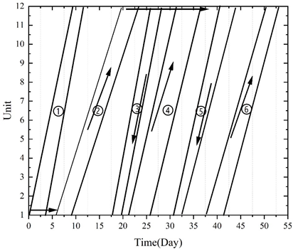
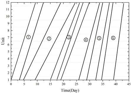
Pipeline engineering is a typical example of a repetitive project. According to the construction sequence of pipeline engineering, it consists of six main processes: pipeline positioning, trench excavation, pipeline socketing, pipeline installation, pressure testing and earth backfilling.
For a 12 km pipeline project, 1 km is one unit and there are 12 units in total. The pipeline project is to be completed within 45 days, with a buffer time of 1 day between adjacent processes and the interval between processes.
Assuming that the daily costs of task forces, equipment, resources, etc. for different processes are 280, 180, 220, 320, 250, and 180, respectively. it can be calculated that the total duration of the critical path of all sub-processes in the first unit is 28 days, and the desired construction rate, the theoretical number of task forces, the actual number of task forces, and the planned construction rate for each process can be obtained by calculating the relevant parameters in the LOB scheduling The calculation is shown in Table 2. The desired construction rate of 3.08 and the number of theoretical teams for each process are calculated to be 1.07, 2.72, 1.05, 3.15, 1.07, 1.61. The number of actual teams is 2, 3, 3, 4, 2, 3. The planned construction rates are 1.1, 0.71, 1.1, 0.71, 1.1, 0.71, 1.1, 0.71, respectively.
| Process | Procedure name | Unit period | Pretightening process | Expected construction rate | Number of theoretical teams | The number of actual teams | Planned rate |
| 1 | Pipeline positioning | 3 | – | 3.08 | 1.07 | 2 | 1.1 |
| 2 | Trench excavation | 6 | 1 | 3.08 | 2.72 | 3 | 0.71 |
| 3 | Pipe socket | 3 | 2 | 3.08 | 1.05 | 3 | 1.1 |
| 4 | Pipeline installation | 8 | 3 | 3.08 | 3.15 | 4 | 0.71 |
| 5 | Pressure test | 3 | 4 | 3.08 | 1.07 | 2 | 1.1 |
| 6 | Soil return | 3 | 5 | 3.08 | 1.61 | 3 | 0.71 |
The theoretical number of task forces calculated by Eq. are not integers, and the number of task forces for each process is rounded upward to obtain the actual number of task forces and the actual construction rate, thus obtaining the LOB scheduling program. According to the above table to draw the project LOB diagram, the number of teams after rounding up the LOB scheduling shown in Figure 4.
In order to be able to complete the project within 45 days of the contract duration, all processes are performed at the desired construction rate. However, the number of teams for each process in this scenario is not an integer, so in the plan scheduling, the number of teams is rounded upward, so the construction rate for each process is increased.
The construction rate of process 1, process 3, and process 5 is increased from 1.1 to 0.71, and that of process 2, process 4, and process 6 is increased to 0.71. The adjusted LOB scheduling plan has a duration of 55 days, which exceeds the contractual duration of the project by 10 days.
Processes 3 and 5 are on the control path, and their construction rates are greater than those of the immediately preceding and immediately following control processes, so they are inverse control processes.
In order to ensure that the deadline meets the project contract duration it is usually necessary to make necessary corrections to the LOB scheduling scheme. Using the branch-and-bound algorithm proposed in this paper for solving the LOB resource allocation problem, i.e., using the resource-adjusted schedule optimization model to re-determine the number of task forces for each process, we obtain a scheduling plan that meets the project schedule with the least increase in task forces.
In order to satisfy the contractual duration of this pipeline project, while ensuring the constraints, the number of task forces to be employed for each of the processes 1, 2, 3, 4, 5, and 6 is 3, 4, 3, 5, 3, 3, and their respective start times are 0, 3.3, 18, 20, 28.2, and 28.7, so that the duration of each of these processes after the transformation is calculated to be 12, 23, 13, 17.1, 12, 12, and the finish time of the last process is 44.3, which satisfies the contractual duration, 13, 17.1, 12, 12. At this point, the end time of the last process is 44.3, which satisfies the contract duration. The LOB diagram under the resource-adjusted scheduling program is shown in Figure 5. After adjusting the number of work teams, the construction rate of process d increases, which diminishes the effect of the inverse control process c. The increased construction rate of process f makes the original inverse control process e no longer an inverse control process. Ultimately, the project can be completed within the contract period and the additional cost due to the adjustment of resources is 2,130.
This paper proposes a resource optimization model in the repetitive project scheduling problem, based on the repetitive project process classification and characteristics of LOB, proposes the relevant constraints that need to be satisfied in the LOB resource allocation problem, and introduces the branching limit algorithm to optimize the LOB resource allocation. A specific construction case is brought in for schedule optimization based on LOB scheduling scheme.
Comparing the performance of the four LOB scheduling methods CPM/LOB, ALISS, RUSS, and SHLOB for randomly generating arithmetic cases, CPM/LOB fails to give feasible solutions for all the cases due to the method’s own defects. When parameter \(\overline{k}_{j}\) is randomly selected from the integer interval [3.5], \(n\)=100, \(\theta\)=0.3, the ratio of finding feasible solutions for ALISS( RUSS) is 0.4296, which shows a clear advantage of ALISS( RUSS) compared with CPM/LOB.
The LOB scheduling method is improved by using the branch limit algorithm, and the optimized LOB resource adjustment model shortens the project duration by adjusting the number of task forces for different control processes, and an integer planning model is established, which can obtain the best resource allocation under the guarantee of continuous distribution of resources, and complete the project requirements in a fixed duration to achieve the optimal allocation of resources.
2021 National Natural Science Foundation of China (General Project): Research on Robust Scheduling of Repetitive Projects Based on Key Process Characteristics (Fund Number: 72171081).