inite element simulation technology is based on the means of software to achieve the calculation, the common modular parameter settings based on the software operation steps are: the initial determination of the type of analysis (to understand what to do), pre-processing of the model structure (basic properties such as materials and mesh delineation), load and solve (simulate the real boundary conditions), and post-processing (to effectively analyze the resultant parameters) [1-3].
Pavement structural layer modulus, as an important design parameter in the design process of road structure, plays a very important role in the decision making of road management, maintenance and repair and reconstruction [4-6].
Currently, in the research of asphalt pavement inverse problems, it is assumed that the asphalt layer is a linear elastic system [7], i.e., the materials of each layer of the pavement are linearly elastic, homogeneous, and isotropic [8]. However, this assumption has a certain deviation from the actual situation, and the asphalt pavement materials actually have nonlinear characteristics of stress-strain [9-10]. Engineering practice has shown that the practicality and accuracy of using the pavement elastic laminate system for design and calculation have been increasingly limited [11,12].
Asphalt mixtures are one of the most commonly used materials in highway pavements [13] and are subjected to dynamic loads from traffic vehicles [14]. It is crucial to analyze the dynamic load response characteristics of asphalt mixtures when designing and evaluating the performance of asphalt pavements [15,16]. Asphalt mixtures exhibit a viscoelastic characteristic when subjected to cyclic dynamic loading, and their mechanical properties are affected by both the internal structure of the material and the external loading [17,18]. The dynamic load response characteristics of asphalt mixtures mainly include its deformation characteristics, stress distribution and other aspects [19]. Under the action of load, asphalt mixtures undergo elastic and plastic deformation [20]. Elastic deformation is recoverable while plastic deformation is not recoverable. The stress distribution, on the other hand, indicates the stresses at different locations within the asphalt mixture, which is important for assessing the stability and life of the pavement structure [21]. Viscoelastic mechanical analysis of asphalt pavement is a method to study the force response of asphalt mixtures, through which the deformation and stress distribution law of asphalt mixtures can be revealed to provide a scientific basis for the design and maintenance of pavements [22,23].
Based on finite element software, this paper establishes a variety of types of asphalt pavement finite element models taking into account the viscoelasticity of asphalt pavements, and designs the material damping of asphalt pavements and related parameters in combination with finite element software, and also designs the loading experimental conditions of different pavement structures. On the basis of analyzing the viscoelastic behavior of the material, the viscoelastic intrinsic model of asphalt pavement is designed, the design process of the inverse problem of viscoelastic mechanics of asphalt pavement is proposed, and the inverse problem is computationally solved by combining the root mean square error. For the change of mechanical properties of viscoelasticity inside asphalt, this paper illustrates the effectiveness of the inverse problem calculation method through the change of modulus of each structural layer and the comparison between the inverse calculation results and the measured results. In addition, the effects of different braking coefficients, temperature fields, and load loading frequency on the asphalt pavement structure are also designed.
With the rapid development of China’s national economy, highway construction has entered a stage of development represented by high-grade highways. As far as the pavement structure of highways is concerned, there are two main categories, namely, asphalt pavement and cement concrete pavement. Among them, the use of asphalt pavement accounts for more than 70%. Asphalt pavement is the main pavement form used in China’s highways, and cement concrete pavement occupies an important position in highways with its unique performance and good durability. In the vehicle load and environmental factors of the long-term role of cement concrete pavement road performance gradually decay, when the pavement performance of flatness, skid resistance and load-bearing capacity and other performance is reduced to the limit of the bottom line standard, or its load-bearing capacity can not meet the traffic demand, asphalt paving layer can be used to repair, to improve the performance of the pavement.
In the ANYSYS finite element analysis model of asphalt pavement, the surface structure is defined by means of the viscoelastic cell Visco89, the subgrade structure is defined by means of the three-dimensional solid cell Solid95 with intermediate nodes selected, and the planar structure is defined by means of the 8-node Plane82 cell. The mesh is divided according to hexahedral division, where the local mesh is degraded to tetrahedral. The schematic diagram of the pavement structure model is shown in Figure 1, where the Y-axis is the vehicle traveling direction, the X-axis is perpendicular to the vehicle traveling direction, and the Z-axis is the depth of the pavement structural layer. The asphalt surface layer is further divided into a number of sublayers to analyze the pavement structural changes at different temperatures.

The pavement is simplified as a rectangular body with length and width of 4m, and the height is determined according to the actual calculation demand. Since the upper load has less influence on the soil particles in the part of the pavement depth below 5 m, the thickness of the soil base is taken as 5 m. In order to realistically simulate the actual stress state of the pavement structure, the boundary conditions are set as the displacement of front and back, left and right and bottom of the fixed model, and the displacement of the top contact surface with the tires is allowed only. Definition of interlayer stress transfer through contact, so set the contact surface between the grass-roots level and the surface layer, using ANSYS finite element software to simulate the interlayer contact, if the rigid body, flexible body contact occurs, the rigid body as the target surface, the flexible body as the contact surface.
Material parameters of asphalt pavement
This study focuses on the response of the conversion parameters obtained from different test methods to the stress field of the asphalt pavement structure. In order to facilitate the study and simulate relatively real road conditions, this paper adopts a unified pavement structure, the surface layer is 5cm upper layer, 7cm middle layer and 9cm lower layer of asphalt pavement typical pavement structure, the grass-roots level is a three-layer cement stabilized gravel, the parameter is taken from the “highway asphalt pavement design specification”. The structure and pavement parameters of asphalt pavement are shown in Table 1, and the friction coefficient between asphalt surface layers is set to 0.8, and the friction coefficient between surface layer and base layer is set to 0.55.
| Road structure and material parameters | ||||
| Structural layer | Thickness | Density | Modulus | Poisson ratio |
| Face layer | 5cm | 2500 kg/m$$^3$$ | Viscoelastic parameter based on CMA model fitting | |
| 7cm | 2400 kg/m$$^3$$ | |||
| 9cm | 2400 kg/m$$^3$$ | |||
| Cement stabilized gravel base | 25cm | 2200 kg/m$$^3$$ | 15000MPa | 0.2 |
| 25cm | 14000MPa | 0.2 | ||
| 25cm | 13000MPa | 0.2 | ||
| Soil base | / | 1600 kg/m$$^3$$ | 50MPa | 0.4 |
Material Damping
Material damping seriously affects the dynamic response of the pavement. Through the ABAQUS program can define a variety of damping forms, this paper according to the specific circumstances of the selection of Rayleigh damping to characterize the structural damping. Compared with other forms of damping, the damping of each order mode of the system can be precisely defined. Assuming that the damping matrix is a linear combination of the mass matrix and stiffness-proportional damping, the:
\[\label{GrindEQ__1_} C=\alpha [M]+\beta [K],\tag{1}\] where \(\alpha\) is the mass damping coefficient and \(\beta\) is the stiffness damping coefficient. According to the vibration orthogonality condition, these two damping coefficients can be calculated from the vibration modes and damping ratios as follows: \[\label{GrindEQ__2_} \alpha =\frac{2\omega _{i} \omega _{j} \left(\omega _{i} \xi _{j} -\omega _{j} \xi _{i} \right)}{\omega _{j}^{2} -\omega _{i}^{2} } ,\beta =\frac{2\left(\omega _{i} \xi _{j} -\omega _{j} \xi _{i} \right)}{\omega _{j}^{2} -\omega _{i}^{2} },\tag{2}\] where \(\omega _{i}\) and \(\omega _{j}\) are the intrinsic frequencies of any two vibration modes, \(\xi _{i}\) and \(\xi _{j}\) are the corresponding damping ratios of the corresponding vibration modes. Generally take the first-order and second-order vibration mode, the damping ratio in a certain frequency range can be approximately constant, the equation can be further simplified as: \[\label{GrindEQ__3_} \alpha =\frac{2\omega _{1} \omega _{2} \xi }{\omega _{1} +\omega _{2} } ,\beta =\frac{2\xi }{\omega _{1} +\omega _{2} } .\tag{3}\]
The modal analysis of the finite element model of the pavement structure was carried out using the Lanczos method in the linear ingress analysis step in ABAQUS/Standard. The first two orders of modes were extracted for the overall pavement structure, which corresponded to the frequencies of 30.028 ad/s and 36.3757 rad/s. The damping ratio of the pavement structure is generally in the range of 0.01 to 0.04, so in this paper, the damping ratio is taken to be 0.03, and the Rayleigh damping coefficient is taken to be \(\alpha =1.628,\beta =0.001\).
The finite element meshing in this calculation uses 8-node reduced integration cell C3D8R, which type of cell can get higher accuracy with smaller computational cost. Among them, the asphalt concrete layer is located in the surface layer of the bed of the structure (taken as 5, 7, and 9 cm thickness respectively). In the calculation, the axle load of the Russian passenger and freight co-located train sets is considered according to the maximal axle weight of 20t, and the single wheel actually exerts the centralized force with the size of 120kN, and the lateral force with the size of 90kN is exerted in the lateral direction. Boundary conditions are considered as a full structural calculation model, at the same time, combined with the depth range of dynamic stress influence of previous studies, in the stage of “joint commissioning” on the Wuhan-Guangzhou line, when the depth of the roadbed is 4 meters, the attenuation rate of dynamic stress and vibration acceleration within the roadbed ranges from 81.52% to 90.09% and from 78.54% to 88.82%, and the attenuation rate below 4 meters is 81.52%\(\mathrm{\sim}\)90.09% and 78.54%\(\mathrm{\sim}\)88.82%, respectively. 88.82%, the stress on the soil base below 4 meters is quite small, so the thickness of the whole roadbed structure is taken as 4 meters.
In terms of boundary conditions, all six degrees of freedom on the bottom surface of the model are constrained, symmetric boundary conditions are imposed on the transverse profiles at the longitudinal ends, i.e., no movement outside the symmetric plane and no rotation inside the symmetric plane can take place, normal displacement constraints are imposed on the transverse ends, and no constraints are imposed on the other free parts.
In addition, the temperature and brake coefficient changes also affect the performance of asphalt pavement, so the same temperature and braking coefficient are maintained in the experiment.
Three-layer asphalt structure in the upper layer is mainly to solve the anti-skid, anti-rutting and smoothness and other functional problems, to provide a safe and comfortable environment for vehicle travel. Middle surface layer in addition to the main rutting resistance, load-bearing and dense waterproof function, but also take into account certain fatigue cracks occurring problems. The following layer and semi-rigid grass-roots level in direct contact, connecting the asphalt surface layer and semi-rigid grass-roots level so that it becomes a whole with a certain degree of strength, also known as the joint layer. According to the stress characteristics of asphalt pavement materials, asphalt pavement structural layers of their respective roles and solve the corresponding functional requirements. Asphalt pavement also has a certain degree of viscoelasticity, the study of its mechanical counterproblems can help to clarify the viscoelasticity of asphalt pavement, in order to optimize and enhance its service life to provide support.
Viscoelastic materials exhibit creep and relaxation mechanical behavior after being loaded, and will exhibit deformation recovery behavior after the load is removed. It is usually considered that when not subjected to external loading, the material is in a state of natural relaxation, at which time the deformation and internal stress of the object are zero. Starting from \(t=0\) time, it is considered that the viscoelastic material is disturbed by external factors, and the stress and strain are both zero.
Creep deformation
At \(t=0\), a constant stress \(\sigma _{0}\) is applied, the resulting strain \(\varepsilon\) increases with \(t\) and its rate of increase decreases with time \(t\), if the magnitude of the stress \(\sigma _{0}\) is increased, the strain \(\varepsilon\) increases with it. For elastic materials, the strain is constant and does not vary with time for a given stress. For viscous flow materials, the strain increases with time and grows uniformly. Creep can be defined as: \[\label{GrindEQ__4_} \varepsilon (t)=\sigma _{0} H(t).\tag{4}\]
The strain response of a viscoelastic material under the stress of creep deformation is: \[\label{GrindEQ__5_} \varepsilon (t)=\sigma _{0} J(t) ,\tag{5}\] where \(J(t)\) is the creep flexibility.
Asphalt mixture is a typical viscoelastic material, its creep characteristics can be divided into three stages, namely, creep migration stage, the strain and time present a nonlinear relationship, and the strain growth rate with the development of time and decrease. Creep stabilization stage, the strain still increases with the development of time, but the rate of change is basically unchanged. Creep damage stage of instantaneous destruction, the strain rate increases rapidly with time.
Stress relaxation
A constant strain \(\varepsilon _{0}\) is applied at \(t=0\), then \(\sigma\) decreases with time. Stress relaxation corresponds to creep, in which the stress in a material decays rapidly from the beginning, with a decreasing rate of decay, eventually decreasing to a value close to a certain value, and the viscous flow decays to zero after a sufficiently long period of time. Under the same \(\varepsilon _{0}\) conditions, the stresses in a solid material will decay to a certain value after a long time, while the stresses in a fluid material will decay to zero more quickly. The stress response under the action of Definition \(\varepsilon (t)=\sigma _{0} J(t)\) is expressed as: \[\label{GrindEQ__6_} \varepsilon (t)=\varepsilon _{0} Y(t),\tag{6}\] where \(Y(t)\) is the relaxation modulus. The stress in the asphalt mixture relaxes very rapidly at the beginning, then the stress relaxation gradually slows down and finally stabilizes slowly.
Strain recovery
After the applied stress \(\sigma _{0}\) is removed, the strain \(\varepsilon\) decreases gradually with the development of time, or in the case of an elastic solid, the strain decreases until it reverts. This phenomenon of gradual increase in the strain of a material under the action of an external force, and gradual decrease in strain until the solid is restored to its original state after the removal of the applied stress is known as delayed elasticity. Factors affecting the delayed elasticity curve include temperature in addition to time.
While the stress and strain of an isotropic linear elastic material are simply linear, the strain of a viscoelastic material is also a function of time in addition to stress. Under the action of constant stress \(\varepsilon (t)=\sigma _{0} \cdot H(t)\), the strain at the moment \(t\) is: \[\label{GrindEQ__7_} \varepsilon (t)=D(t)\cdot \sigma _{0} ,\tag{7}\] where \(\varepsilon (t)\) is the strain with respect to time, \(\sigma _{0}\) is the amplitude of the constant stress. \(H(t)\) is the step function, i.e: \[\label{GrindEQ__8_} H(t)=\left\{\begin{array}{l} {0,t\le 0^{-} } \\ {1,t\ge 0^{+} } \end{array}\right.\tag{8}\]
Eq. (7) is the applied constant stress carried out at moment 0. If the stress is applied at moment \(\tau\) with constant force \(\sigma (t)=\sigma _{0} \cdot H(t-\tau )\), Eq. (7) can be expressed as: \[\label{GrindEQ__9_} \varepsilon (t)=\left\{\begin{array}{l} {0,t<\tau } \\ {D(t-\tau ),t\ge \tau } \end{array}\right.\tag{9}\]
Any stress function \(\sigma (t)\) can be decomposed approximately in the form of a superposition with a series of constant forces, i.e., a constant force \(\sigma _{0}\) acting at moment 0, a constant force acting at moment \(\tau _{1}\) a constant force acting at moment \(\Delta \sigma _{1} ,\tau _{2}\) a constant force acting at moment \(\Delta \sigma _{2} ,\ldots ,\tau _{n}\) a constant force acting at moment \(\Delta \sigma _{n}\). Thus, the strain at moment \(t\) can be expressed as: \[\label{GrindEQ__10_} \varepsilon (t)=D(t)\cdot \sigma _{0} +\sum _{i=1}^{n}D \left(t-\tau _{i} \right)\cdot \Delta \sigma _{i} .\tag{10}\]
In fact, Eqs. (7) and (9) are only for constant loads in an ideal state. In engineering, the load application process can seldom be regarded as instantaneous, and the change of load and the deformation of the material itself will also make the stress change. Therefore, in engineering applications, it is more important for the viscoelastic model to be able to solve the strain function \(\varepsilon (t)\) under an arbitrary stress function \(\sigma (t)\). Using the idea of approximation, the stress function can be divided into a number of time segments in time, and each time segment is regarded as a constant stress, and the amplitude of the stress at the beginning of the time segment is taken as the amplitude of the constant stress at that time. In this way, an arbitrary stress function can be divided into the form of a number of constant stress superposition, so as to better carry out the calculation of viscoelastic energy.
In the theory of viscoelasticity, different viscoelastic models can be composed of two basic elements, the viscous pot and the spring, and the mechanical response of the material can be determined according to the relaxation function and creep flexibility of the model. Its corresponding stress-strain relationship obeys the linear Hookean’s law, and has the obvious characteristics of instantaneous elastic deformation and instantaneous recovery, i.e.: \[\label{GrindEQ__11_} \sigma =E\varepsilon,\tag{11}\] where \(\sigma\) is the stress, \(\varepsilon\) is the strain, and \(E\) is the Young’s modulus of the spring.
The relationship between stress and strain corresponding to the viscous kettle element obeys the law of viscosity, i.e., there is a linear relationship between the strain rate and the stress. Then: \[\label{GrindEQ__12_} \sigma =\eta \dot{\varepsilon } ,\tag{12}\] where \(\dot{\varepsilon }\) is the strain rate and \(\eta\) is the coefficient of the sticky pot.
When the Heaviside stress acts on the sticky pot, the strain rate is obtained as: \[\label{GrindEQ__13_} \dot{\varepsilon }=\frac{\sigma _{0} }{\eta } .\tag{13}\]
Integrating the above equation yields: \[\label{GrindEQ__14_} \varepsilon =\frac{\sigma _{0} }{\eta } t .\tag{14}\]
A basic two-element mechanical model, i.e., the Maxwell model, is obtained by combining the sticky pot element and the spring element in series.
Based on the basic physical theory of equal cross-section stresses, the total strain \((\varepsilon )\) corresponding to the Maxwell model is the sum of the strain of the spring element and the strain of the sticky pot element, that is: \[\label{GrindEQ__15_} \varepsilon =\varepsilon _{1} +\varepsilon _{2} ,\tag{15}\] where \(\varepsilon _{1}\) is the spring element strain and \(\varepsilon _{2}\) is the sticky pot element strain.
According to the above formula can be obtained: \[\label{GrindEQ__16_} \sigma +\frac{\eta }{E} \dot{\sigma }=\eta \dot{\varepsilon } .\tag{16}\]
After applying stress \(\sigma =\sigma _{0} H(t)\), the total strain of the Maxwell model is equal to the sum of the spring element strain and the viscous pot element strain, i.e.: \[\label{GrindEQ__17_} \varepsilon =\frac{\sigma _{0} }{E} \left(1+\frac{E}{\eta } t\right)=\frac{\sigma _{0} }{E} +\frac{\sigma _{0} }{\eta } t .\tag{17}\]
The corresponding creep function is: \[\label{GrindEQ__18_} J(t)=\frac{1}{E} +\frac{t}{\eta } ,\tag{18}\] after applying a constant strain \(\varepsilon _{0}\) to the Maxwell model: \[\label{GrindEQ__19_} \sigma (t)=E\varepsilon _{0} e^{-\frac{t}{\tau _{i} } } ,\tag{19}\] where \(\tau _{i}\) is the relaxation time and is equal to \(\eta /E\).
The corresponding relaxation function is: \[\label{GrindEQ__20_} G(t)=Ee^{-\frac{t}{\tau _{i} } } .\tag{20}\] Because the relaxation function tends to 0 at \(t\to \infty\), the Maxwell model is essentially a viscoelastic fluid model, which is directly used to describe the viscoelastic mechanical response of asphalt and asphalt mixtures with large errors.
By combining the viscous and elastic elements in parallel, another basic two-element mechanical model is obtained, i.e., the Kelvin model.
Under the combination of parallel connection, the stresses of the viscous element and the elastic element are independent of each other and the strains are the same, i.e., the total stress \((\sigma )\) corresponding to the Kelvin model is the sum of the elastic element strain \(\left(\sigma _{1} \right)\) and the viscous element strain \(\left(\sigma _{2} \right)\), and then: \[\label{GrindEQ__21_} \sigma =\sigma _{1} +\sigma _{2} =E\varepsilon +\eta \dot{\varepsilon } .\tag{21}\] When the stress \(\sigma =\sigma _{0} H(t)\) acts on the model structure, at \(t>0\) time \(\sigma =\sigma _{0} ,\dot{\sigma }=0\), the eigenstructure equation at this point can be written as: \[\label{GrindEQ__22_} E\varepsilon +\eta \dot{\varepsilon }=\sigma _{0} .\tag{22}\] The above equation can be written as: \[\label{GrindEQ__23_} \varepsilon =\frac{\sigma _{0} }{E} \left(1-e^{\frac{t}{\tau _{d} } } \right) ,\tag{23}\] where \(\tau _{d} =\frac{\eta }{E}\) is the delay time.
By combining the Kelvin model and the Maxwell model in a series fashion, a four-element mechanical model, the Burgers model, is obtained.
The eigenstructure equation of the Burgers model is: \[\label{GrindEQ__24_} \sigma +p_{1} \dot{\sigma }+p_{2} \ddot{\sigma }=q_{1} \dot{\varepsilon }+q_{2} \ddot{\varepsilon },\tag{24}\] where \(p_{1} =\frac{\left(\eta _{1} E_{1} +\eta _{1} E_{0} +\eta _{0} E_{1} \right)}{E_{1} E_{0}} ;\) \(p_{2} =\frac{\eta _{1} \eta _{0}}{E_{1} E_{0}} ;\) \(q_{1} =\eta _{1} ;\) and \(q_{2} =\eta _{1} \eta _{0} /E_{0}\).
Solving the above equation yields the strain response when the constant stress \(\sigma =\sigma _{0} H(t)\) acts on the model structure: \[\label{GrindEQ__25_} \varepsilon (t)=\sigma _{0} \left[\frac{1}{E_{1} } +\frac{t}{\eta _{1} } +\frac{1}{E_{0} } \left(1-e^{-\lambda t} \right)\right],\tag{25}\] where \(\lambda =\frac{E_{2}}{\eta _{2}}\).
Then the creep function is: \[\label{GrindEQ__26_} J(t)=\frac{1}{E_{1} } +\frac{t}{\eta _{1} } +\frac{1}{E_{0} } \left(1-e^{-\lambda t} \right) .\tag{26}\] The relaxation stress of the Burgers model can be written as: \[\label{GrindEQ__27_} \sigma (t)=\frac{\varepsilon _{0} }{\sqrt{p_{1}^{2} -4p_{2} } } \left[\left(-q_{1} +\alpha q_{2} \right)e^{-\lambda t} +\left(q_{1} -\beta q_{2} \right)e^{-\beta t} \right] ,\tag{27}\] where \(\alpha =\frac{1}{2p_{2} } \left(p_{1} +\sqrt{p_{1}^{2} -4p_{2} } \right)\) and \(\beta =\frac{1}{2p_{2} } \left(p_{1} \sqrt{p_{1}^{2} -4p_{2} } \right)\).
Then the relaxation function is: \[\label{GrindEQ__28_} G(t)=\frac{1}{\sqrt{p_{1}^{2} -4p_{2} } } \left[\left(-q_{1} +\alpha q_{2} \right)e^{-\lambda t} +\left(q_{1} -\beta q_{2} \right)e^{-\beta t} \right] .\tag{28}\]
The Burgers model has a moderate number of model parameters, its mechanical model derivation process is relatively simple, and the model has been popularized to a certain extent in engineering applications. By correcting the tandem pots in the Burgers model, different types of deformations of asphalt and asphalt mixtures can be accurately described. The traditional modified Burgers model adopts an exponential form to modify the tandem sticky pots, which cannot accurately describe the deformation law of creep in the third stage. Therefore, this study will use the binary function to modify the tandem viscous pots, thus analyzing the inverse problem calculation of the viscoelastic mechanical response of asphalt pavement.
The inverse problem design process established in this paper is mainly composed of three parts: asphalt pavement performance analysis, positive problem computation and inverse problem computation, which are functionally independent of each other, and the inverse problem design process for the viscoelastic mechanics of asphalt pavement is shown in Figure 2. Among them, the asphalt pavement performance analysis is used to extract the mechanical changes corresponding to the asphalt pavement to be designed by the inverse problem, and the main role of the positive problem computation is to generate the computational domain mesh and update the corresponding force field under the current asphalt pavement. The inverse problem computation is to determine whether the current inverse problem design converges or not, and in case of non-convergence, to extract the required parameters such as the mechanical response of the asphalt pavement surface from the numerical results of the force field obtained from the previous inverse problem computation. Combined with the inverse problem calculation method to solve the mechanical response deformation of asphalt pavement at each place, to get the updated mechanical response of asphalt pavement results.

This paper adopts the asphalt pavement viscoelastic mechanics backcalculation method is in the review of a large number of literature based on the determination of the initial parameters of each layer of material, the use of finite element software ABAQUS for positive calculation, the calculated results will be obtained and the actual results obtained from the test for comparison, and then gradually modify the parameters of each layer for iterative calculations, when the calculated results and the actual results of the root-mean-square error between the minimum hours, the end of the iterative process. Then: \[\label{GrindEQ__29_} e=\sqrt{\frac{\sum _{i=1}^{n}[(l_{i}^{0} -l_{i}^{j} )/l_{i}^{0} ]^{2} }{n} } ,\tag{29}\] where \(e\) is the root mean square error, \(l_{i}^{0}\) is the measured bending, \(l_{i}^{j}\) is the calculated bending, and \(n\) is the number of measurement points.
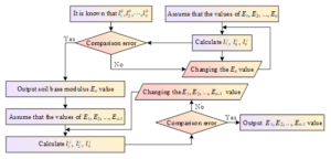
For each layer modulus of the pavement structure, the roadbed modulus occupies an important position in the whole backcalculation process, which directly affects the accuracy of the backcalculated values of other layers modulus. In this paper, the modulus of roadbed is firstly determined by the bending values of 4 measurement points after the bending basin, and then the modulus of roadbed is changed to the modulus of roadbed obtained by backcalculation, and the modulus of other structural layers is backcalculated according to the bending values of all the 10 measurement points in order from bottom to top. The specific inverse calculation method is as follows:
Establish the finite element positive calculation model, input the initial modulus, and carry out the finite element positive analysis.
Extract the displacement of each measurement point, compare it with the displacement of each measurement point measured by FWD, and calculate the error, if the error of the last 4 measurement points meets the requirement of accuracy, then the roadbed modulus can be output to carry out the next stage of calculation, or else re-input the roadbed modulus and repeat the operation until the error of the last 4 measurement points meets the requirement of accuracy.
Change the modulus of the roadbed to the modulus of the roadbed after backcalculation, gradually change the modulus of the other structural layers, carry out the calculation, and then extract the displacements of each measurement point and carry out the calculation of the error, and if the error meets the requirement of accuracy, then the modulus can be output and exit the calculation. Otherwise, continue to change the modulus until the error meets the accuracy requirements.
Combining the above steps, the computational flow of the inverse problem of viscoelastic mechanics of asphalt pavement is obtained as shown in Figure 3.
With the strong investment in transportation infrastructure construction, the mileage of high-grade highways increases year by year. As a jointless and continuous pavement structure, asphalt pavement has many advantages, such as good driving comfort, low dust and noise, and easy milling construction, etc. It is widely used in road construction, and is the preferred form of high-grade pavement surface structure at present. However, most of the actual service life of asphalt pavement is far from reaching its design life, and it has to be overhauled or even rebuilt at the early stage of traffic. There are many reasons why the actual serviceability of asphalt pavements fails to meet the expected purpose, such as harsh climatic environment, serious overloading phenomenon, and defects in asphalt mixture design and construction. The large-scale and high-frequency early damage phenomenon not only reduces the service life of asphalt pavement and increases the construction and maintenance costs, but also has a very great impact on the harmonious development of society and economy.
Based on the finite element model established in this paper for the analysis of three-dimensional viscoelastic mechanics inverse problem of asphalt pavement, taking 10t load as the basic load, three different pavement structures were set up to carry out the inverse computation, and the inverse problem computation results of the modulus of each layer of the different pavement structures were obtained as shown in Table 2.
For pavement structure 1, pavement structure 2, and pavement structure 3, four of the materials in each layer of the three pavement structures are the same, which are SBS-AC20 asphalt concrete, cement-stabilized graded gravel, cement-stabilized soil, and soil base. According to the data in the table, it can be seen that the calculated modulus of the inverse problem of SBS-AC20 asphalt concrete corresponding to the three types of pavement structures are 2060 MPa, 2400 MPa, and 2320 MPa, respectively, with a maximum relative error of 5.26%. The maximum relative errors of the calculated modulus of the inverse problem corresponding to the three pavement structures were 5.63%, 5.88% and 4.65% for cement stabilized graded gravel, cement stabilized soil and soil base, respectively, and the maximum relative errors were all within 6%. It can be seen that the results of their inverse problem calculation modulus for the same materials are more consistent, indicating that the inverse problem calculation method proposed in this paper is feasible to be applied in the calculation of the inverse problem of viscoelastic mechanics of asphalt pavements.
| Pavement structure | The modulus is the result of the problem | ||
|---|---|---|---|
| Road structure 1 | Road structure 2 | Road structure 3 | |
| SBS-AC15 | – | 1650MPa | – |
| SBS-AC20 | 2280MPa | 2400MPa | 2320MPa |
| SBS-AC25 | 1100MPa | – | 1200MPa |
| SBS-AC30 | – | 2565MPa | 2200MPa |
| Cement stabilized with gravel | 1460MPa | 1500MPa | 1420MPa |
| Cement stabilizer | 680MPa | 720MPa | 690MPa |
| Soil base | 45MPa | 44MPa | 42MPa |
Replace the initial modulus of each layer in the original finite element model with the calculated modulus of the inverse problem of each layer under 10t load, and carry out the calculation and analysis. Pavement structure 1 and pavement structure 2 are selected to compare the actual and calculated bending settlement results of asphalt pavement under two different loads of 15t and 20t, respectively, and the comparison results under different loading conditions are obtained as shown in Figure 4. Among them, Figure 4(a) and (b) show the comparison results between calculated and measured under 15t and 20t loads, respectively.
In Figure 4(a), the measured deflection value and the calculated deflection value of the two asphalt pavement structures in each measurement point under 15t load gradually decrease with the increase of the distance from the load, and when the distance from the load is about 1.8 meters, the relative error between the measured deflection value and the calculated deflection value of the two pavement structures is 4.23% and 1.62%, respectively. It can be seen that the calculated deflection basin of each measurement point and the measured deflection basin are well matched, and the calculated deflection value of each measurement point is in good agreement with the measured deflection value.
In Figure 4(b), the curves of measured and calculated bending settlements of the two asphalt pavement structures under 20t load are similar to those under 15t load, and the calculated bending settlements of the two different asphalt pavement structures are closer to the measured bending settlements. When the distance from the load is 0.3m, the maximum relative error between the calculated and measured values is 12.65%, and when the distance from the load is 0.4m, the maximum relative error is 4.22% for the pavement structure 2.
With the enhancement of the loading effect, the bending trend shown by the asphalt pavement is closer, which also reflects that this paper can clarify the bending trend of the asphalt pavement subjected to external loading by the way of inverse problem calculations, and provide support for the optimization of the viscoelastic mechanics of the asphalt pavement.

Asphalt pavement in the use of the process will be affected by the braking of the vehicle driving process, tires on the pavement not only vertical load, due to the tire and pavement friction with each other caused by the horizontal load, the existence of horizontal load on the asphalt pavement damage is also very large. Therefore, this paper gives full consideration to the influence of different braking coefficients on asphalt pavement shear stress in the case of vehicle moving load. The temperature field of asphalt pavement under high temperature in summer is taken as the test environment, and the braking coefficients are set as 0, 0.2, 0.4 and 0.6 respectively to study the change of shear stress of asphalt pavement. Figure 5 shows the shear stress changes of asphalt pavement under different braking coefficients, where Figure 5(a)\(\mathrm{\sim}\)(d) shows the shear stress changes with braking coefficients of 0, 0.2, 0.4, and 0.6, respectively.
When the braking coefficient is 0, the shear stress of each structural layer of the pavement under the action of the moving load, each layer has experienced two horizontal shear stresses in the opposite direction, the asphalt surface layer of negative shear stress according to the value of the size of the location of the asphalt surface layer below 5cm, 12cm, 5cm, asphalt surface layer at the bottom of the layer of the shear stress is almost 0. Positive shear stress according to the value of the size of the asphalt surface layer in the order of the position is 12cm and 5cm below the asphalt surface layer. 5cm and 12cm of the asphalt surface layer, the shear stress is positive and negative alternating changes, so the middle surface layer is not only subjected to large shear stress, and the shear stress is positive and negative alternating changes, it is easy to produce due to shear fatigue caused by the destruction of the middle surface layer.
When the braking coefficient is 0.2, the negative shear stress at 5cm, 5cm, and 12cm below the pavement layer increases, the positive shear stress at 5cm below the pavement no longer exists, and the positive shear stress at 12cm is reduced by also from 0.045MPa to 0.013MPa.
When the braking coefficient is 0.4, the negative maximum shear stress appears in the location of the change, from the original road surface below 5cm to the road surface below 5cm, the value reached -0.19MPa, there is no longer a positive shear stress in the asphalt surface layer.
When the braking coefficient is 0.6, the law of change of shear stress in each layer is similar to the law of shear stress when the braking coefficient is 0.4, and the maximum value of the negative shear stress in the asphalt layer is further increased to -0.337MPa. 50 and 80cm distances below the pavement layer are affected less by the change of the braking coefficient.
In conclusion, the negative maximum value of asphalt pavement shear stress in the range of 12cm below the road surface and road surface increases with the increase of braking force coefficient, which makes the pavement portion more prone to shear damage. It also proves that when the braking force coefficient increases to 0.4, 0.6, the negative maximum value of asphalt pavement shear stress occurs in the location of 5cm below the road surface changes to 5cm below the road surface. through the analysis of shear stress under the action of mobile load with different braking coefficient, it shows that asphalt pavement structure under the action of dynamic load, there is a very complex stress, accurate analysis of stress, deformation change rule is clear that the pavement occurred The key to the mechanism of damage.

The structural mechanical response of asphalt pavement is affected by the continuous change of the external natural environment, in which the temperature is the most considered factor in the pavement design, high-temperature vehicle withdrawal, low-temperature cracking is a typical type of damage greatly affected by temperature. In order to analyze the stress and deformation of asphalt pavement under the joint action of asphalt pavement temperature field and mobile load under different temperature conditions, the braking coefficient is set to be 0, the vertical load is 0.5MPa, and the traveling speed is 100m/s. The temperature field of summer T1 at noon, and the temperature field of different time periods in winter are taken as the typical temperature field for the analysis of the structural dynamic response of the pavement, and the temperature fields of T2, T3, and T4 are taken as the typical winter three kinds of temperature cycles. 24h temperature cycles, and the temperature decreases sequentially, with the highest temperature in T2 and the lowest temperature in T4. The transverse stress change of asphalt pavement is selected as the research content, and the transverse stress change of asphalt pavement under different temperature fields is obtained as shown in Figure 6, in which Figure 6(a)(b) shows the results of transverse stress change of the ground surface and 20cm below the road marking, respectively.
When the braking coefficient is 0, the maximum transverse compressive stress occurs at the surface layer of the asphalt pavement, and the maximum transverse tensile stress occurs 20 cm below from the asphalt pavement, so the effects of the temperature field on the transverse stresses at these two special locations are investigated separately. Both positive and negative transverse stress maxima of asphalt pavement increase with the decrease of temperature field temperature. When the temperature will be reduced from T1 (12:00 moments in summer) to T4 (T4-18:00 moments), the maximum value of transverse stress of asphalt pavement increases from 0.229 to 0.946, and its maximum value increases 3.13 times. The tensile stress at the bottom of the asphalt surface layer increases sharply when the temperature of the asphalt pavement decreases, which increases the possibility of cracking at the bottom of the asphalt layer and provides an opportunity for pavement cracking. For cold winter areas, asphalt mixtures must provide sufficient tensile strength to resist the lateral stresses generated by cooling to prevent cracking at the bottom of the asphalt layer and resulting in pavement cracks.

The effects of the previous section on the viscoelastic mechanics of asphalt pavements are based on the analysis under fixed load, and this subsection selects the temperature field conditions of 20\(\mathrm{{}^\circ}\)C, 30\(\mathrm{{}^\circ}\)C, 40\(\mathrm{{}^\circ}\)C, and 50\(\mathrm{{}^\circ}\)C for the experiments to explore the changes in the viscoelastic mechanical properties of asphalt pavements analyzed under different load loading frequencies, respectively. Figure 7 shows the influence laws of different loading frequencies on asphalt pavement, where Figures 7(a) and (b) are the influence laws on dynamic modulus and phase angle of asphalt pavement, respectively.
In Figure 7(a), it reflects that the temperature has no obvious effect on the change of dynamic modulus of asphalt pavement, in different temperature environments, the dynamic modulus of the mixture are increased with the increase of the load loading frequency, in the smaller load loading frequency, the difference of dynamic modulus is small, in the larger load loading frequency, that is, when the load loading frequency is more than 10Hz, the lower the temperature do cause the dynamic modulus of the asphalt pavement The greater the dynamic modulus, when the load loading frequency is 20Hz, the dynamic modulus obtained at 20\(\mathtt{{}^\circ\!{C}}\) is 2.33 times higher than that at 50\(\mathtt{{}^\circ\!{C}}\), and the difference in dynamic modulus is larger. Under the same temperature conditions, the dynamic modulus of the asphalt mixture decreases with increasing temperature, and the magnitude decreases continuously. In Figure 7(b), it reflects that the change rule of phase angle of asphalt pavement is the same under different temperature conditions. In the load loading frequency is not greater than 8Hz, the phase angle shows a trend of logarithmic increase. In the loading frequency is greater than 8Hz, the phase angle is a linear decrease in the trend, in the smaller load loading frequency (loading frequency is not greater than 1Hz), the phase angle difference is smaller, in the larger load loading frequency, the phase angle difference is larger. The phase angle of asphalt pavement phase shrinks with the temperature increase at the same load loading frequency, and the shrinkage becomes lower gradually.

In this paper, a finite element model of asphalt pavement was established on the basis of considering viscoelasticity, the inverse calculation method of structural modulus of viscoelastic pavement was studied, the inverse calculation of different pavement structures was analyzed through the viscoelastic intrinsic model, the inverse calculation of the results of the inverse calculation was compared, and the mechanical changes of the asphalt pavement were also studied.
The inverse problem calculated moduli of SBS-AC20 asphalt concrete corresponding to the three types of pavement structures in each layer of the three types of pavement structures are 2060 MPa, 2400 MPa, and 2320 MPa, respectively, with a maximum relative error of 5.26%. The maximum relative error of the inverse computed modulus for each type of pavement structure remains within 6%. The results of the modulus backcalculation obtained under the same material are in good agreement, which indicates the feasibility of the backcalculation method designed in this paper in carrying out the research on the inverse problem of the viscoelastic mechanics of asphalt pavements.
Under 15t load, when the distance from the load is 1.8m, the relative errors between the measured and calculated bending settlement values of the two pavement structures are 4.23% and 1.62% respectively, and the maximum relative error under 20t load is 12.65%. The trend of bending settlement obtained by relying on the inverse calculation method is more consistent with the actual trend.
The negative shear stress of asphalt pavement increases with the increase of braking factor, and its maximum value increases by 3.13 times when the temperature of asphalt pavement decreases from 12:00 in summer to 18:00 in winter. When the load loading frequency is 20Hz, the dynamic modulus obtained at 20\(\mathtt{{}^\circ\!{C}}\) is 2.33 times higher than that at 50\(\mathtt{{}^\circ\!{C}}\). And the phase angle of the asphalt pavement shows a logarithmic increasing trend when the load loading frequency is lower than 8Hz, and shows a linear decreasing trend when it exceeds 8Hz.