Crude oil is a vital bulk energy product, often described as the lifeblood of modern industry. As an essential industrial raw material, it possesses commodity attributes in the general sense [1-2]. In recent years, due to the elevated status and share of crude oil futures in the international commodity market, coupled with the scarcity of oil resources, crude oil has become the focal point of national and regional interests, with its financial and political attributes becoming increasingly prominent [3-4]. However, changes in crude oil prices are often unpredictable. After the 2008 financial crisis, international oil prices experienced frequent and volatile fluctuations. In 2020, the global epidemic outbreak led to a decline in oil demand, which further resulted in a plunge of oil prices, with WTI crude oil futures dropping to a low of -37.6 dollars, triggering panic in the global market [5]. Evidently, crude oil prices are influenced not only by supply and demand but also by geopolitics, emergencies, and other unquantifiable factors, making forecasting work complex but strategically important [6]. For countries, reliable prediction of crude oil prices can grasp national economic development trends, while for industries, it can ensure stable development across various sectors. Therefore, the analysis and prediction of the international crude oil market has become a core concern for relevant departments in China. Government departments, enterprises, and investment institutions are eager to make accurate predictions of international crude oil price trends to facilitate scientific policy-making, production investment, and purchase and sale transactions, while also mitigating risks to the greatest extent possible [7-8].
As the largest developing country globally, China’s economy has been on an upward trend, resulting in an increased demand for crude oil and its ancillary products across various industries. Furthermore, the fluctuations in crude oil prices have a significant impact on global economic development. Consequently, analyzing and forecasting the international crude oil market and crude oil prices becomes crucial. Literature [9] proposed a prediction framework for crude oil prices using a transfer learning approach with long and short-term memory networks as the core logic. This framework demonstrated good generalization ability and prediction accuracy in simulation tests and practical applications. Based on the heterogeneous autoregressive (HAR) analytical framework, literature [10] conducted out-of-sample forecasting for heating oil spot and futures prices using monthly realized variances. The study highlighted that both El Niño and La Niña events significantly influence the values of realized variances. Literature [11] combined six real oil price forecasting systems mentioned in the Journal of Business and Economic Statistics with a futures model. The empirical analysis revealed that the proposed forecasting scheme effectively enhances the accuracy of oil price forecasts. Literature [12] introduced the loss function method into the research framework of oil price prediction and proposed an oil price prediction model based on the empirical genetic algorithm (GPEGA). Compared to the GPGA prediction model, the GPEGA-based model showed improved prediction accuracy and stability. Literature [13] conducted a comparative test to analyze the performance difference between multi-model and single-model approaches in crude oil price prediction. The analysis results indicated that the multi-model crude oil price prediction framework outperforms the single-model approach in terms of comprehensive performance. Literature [14] explored the predictive performance of crude oil price volatility predictors based on the model confidence set (MCS) and found that financial predictors are the most significant factors affecting oil prices. This provides valuable insights and references for managers in the crude oil market. Literature [15] employed multivariate heterogeneous autoregression to establish a volatility analysis framework to investigate how information and correlation between oil futures and the U.S. financial market affect oil price volatility. The study validated the excellent predictive performance of the HAR framework and emphasized the impact of stock market volatility information on oil prices. Literature [16] discussed the differences in time series information between analysts’ assessments of natural gas and oil reserves and highlighted that the level of analysts’ analysis significantly influences the volatility of natural gas and oil prices.
In this paper, we first derive the generalized linear model for logistic regression and obtain the objective function using the maximum likelihood method. Subsequently, the basic framework of the improved logistic regression model is constructed. Optimization is carried out by comparing the convergence speeds of different improved algorithms with conventional algorithms, considering both row and column dimensions of the dataset. Thereafter, the proximal gradient descent method for solving Lasso is introduced. Using the improved model, we construct a logistic-based international oil price prediction model. This model, along with five other logistic regression models, is trained using the dataset. We then compare their performance in predicting international crude oil prices, specifically focusing on the prediction of international crude oil prices under unexpected events such as natural disasters and important data exceeding expectations.
Logistic models are statistically based learning models have a good statistical basis and interpretability. It is derived from exponential family. Definition of exponential family: \[\label{GrindEQ__1_} p(y;\eta )=b(y)\exp \left(\eta ^{T} T(y)-a(\eta )\right) ,\tag{1}\] where \(\eta\) is a characteristic parameter of the distribution, \(T(y)\) is a sufficient statistic for the distribution under consideration, and in general \(T(y)=y,a(\eta )\) is known as the log partition function usually \(e^{-a(\eta )}\) plays an important role in normalizing the parameters, which ensures that the integral or sum of the distribution \(p(y;\eta )\) with respect to \(y\) is equal to one.
For selected \(T,a\) and \(b\) two functions determine the kind of family the distribution belongs to. Consider first the Bernoulli distribution.
The Bernoulli distribution is often also called the binomial distribution, and the Bernoulli distribution with mean \(\phi\) is written \(B(\phi )\), and from Bernoulli’s distribution we know that \(y\in \{ 0,1\}\), and therefore \(p(y=1;\phi )=\phi\). \(p(y=0;\phi )=1-\phi\), and when \(\phi\) is changed a different Bernoulli distribution is obtained, such that: \[\label{GrindEQ__2_} \left\{\begin{array}{l} {T(y)=y}, \\ {a(\eta )=-\log (1-\phi )=\log \left(1+e^{\eta } \right)}, \\ {b(y)=1}. \end{array}\right. \tag{2}\] Is obtained by bringing in Eq. (1): \[\label{GrindEQ__3_} \begin{array}{rcl} {p(y;\phi )} & {=} & {\exp \left(\log \left(\frac{\phi }{1-\phi } \right)y+\log (1-\phi )\right)} \\ {} & {=} & {\exp (y\log \phi +(1-y)\log (1-\phi ))} \\ {} & {=} & {\phi ^{y} (1-\phi )^{1-y} } .\end{array} \tag{3}\] A comparison reveals that Eq. (3) is exactly Bernoulli’s distribution formula, and therefore the Bernoulli distribution belongs to the exponential family.
The following is a discussion of the Gaussian distribution, which is also called the normal distribution and is usually denoted as \(N\left(\mu ,\sigma ^{2} \right)\), where \(\mu\) is called the expected value of the distribution and \(\sigma ^{2}\) is called the variance, and together they both determine the shape of the normal distribution. Let: \[\label{GrindEQ__4_} \left\{\begin{array}{l} {\mu =\eta }, \\ {T(y)=y}, \\ {a(\eta )=\mu ^{2} /2=\eta ^{2} /2}, \\ {b(y)=(1/\sqrt{2\pi } )\exp \left(-y^{2} /2\right)}. \end{array}\right. \tag{4}\] It’s available, \[\label{GrindEQ__5_} \begin{array}{rcl} {p(y;\mu )} & {=} & {\frac{1}{\sqrt{2\pi } } \exp \left(-\frac{1}{2} y^{2} \right)\exp \left(\mu y-\frac{1}{2} \mu ^{2} \right)} \\ {} & {=} & {\frac{1}{\sqrt{2\pi } } \left(-\frac{1}{2} (y-\mu )^{2} \right)}. \end{array} \tag{5}\] Eq. (5) is precisely the distribution function of the Gaussian distribution, and thus the Gaussian distribution also belongs to the exponential family.
Typically, problems of exponential families can be solved by constructing a generalized linear model, and the following assumptions about the conditional probability \(p(y|x;\theta )\) of \(y\) are given for how to construct a generalized linear model, given sample \(x\) and parameter \(\theta\):
\(y|x;\theta\) belongs to the exponential family.
For a given \(x\), the objective is to predict the expectation of \(T(y)\) i.e. \(h(x)=E[y|x]\) here \(T(y)=y\).
\(\eta =\theta ^{T} x\), i.e., \(\eta\) and \(x\) are linearly related.
With the assumptions as above, the general linear regression and Logistic can be constructed, in the general linear regression it is assumed that given the sample \(x\) and parameter \(\theta\), the conditional probability about \(y\) obeys a Gaussian distribution i.e., \(y|x;\theta \sim N\left(\mu ,\sigma ^{2} \right)\), and the first assumption is satisfied by the previous relationship between the Gaussian distribution and the exponential family. According to assumptions (b) and (c) and the nature of the Gaussian distribution can be obtained as, \[\label{GrindEQ__6_} h_{\theta } (x)=E[y|x]=\mu =\eta =\theta ^{T} x . \tag{6}\] While in Logistic, it is assumed that the conditional probability of \(y\) given sample \(x\) and parameter \(\theta\) obeys the Bernoulli distribution i.e. \(y|x;\theta \sim B(\phi )\), from the previous relationship between the Bernoulli distribution and the exponential family it can be seen that the first assumption is fulfilled, in accordance with the assumptions (b) and (c) as well as the nature of the Bernoulli distribution can be obtained by, \[\label{GrindEQ__7_} h_{\theta } (x)=E[y|x]=\phi =1/\left(1+e^{-\eta } \right)=1/\left(1+e^{-\theta ^{T} x} \right) . \tag{7}\] So far, Eq. (6) has been obtained using Gaussian distribution with generalized linear model and Eq. (7) has been obtained using Bernoulli distribution with generalized linear model both of them have a high degree of formal similarity, these two models are the general linear model and the Logistic model, where Eq. (7) is also known as the predictive function of Logistic.
The regression problem is a curve fitting process where a set of curve parameters are computed to make the sample data fit as well as possible on the desired curve. In practice, the curves are not chosen randomly and aimlessly, but the form of the curves, such as straight lines, quadratic curves, etc., is usually assumed first, and then the parameters are learned through computation.
There are two problems in the parameter learning process one is whether the initial assumptions reflect the characteristics of the problem, if you choose to use a straight line to fit a non-linear problem, there will be a major error. The other is whether the curve fit is good or not, if the parameters sought are not ideal, there will be underfitting or overfitting and the results obtained will not be satisfactory.
Assuming that the regression can be performed using a linear model, the linear form of the general linear regression in the plane is obtained according to Eq. (6): \[\label{GrindEQ__8_} y=\theta _{0} +\theta _{1} x_{1} +\theta _{2} x_{2} +\theta _{3} x_{3} +\ldots +\theta _{n} x_{n} , \tag{8}\] where \(x_{i}\) denotes the input component of the model, i.e., the specific value in the sample, and \(\theta _{i}\) is the learning parameter. However, there are following drawbacks of using this model in reality.
Many types of inputs to the model exist, such as continuous values, discrete values, and enumerated values. And the range of values of the inputs varies greatly. For example, the range of outdoor temperature [-50,50], the range of a certain probability [0,1], and so on. Inputs with large ranges tend to make the role of inputs with small ranges negligible in the calculation process. Moreover, linear regression remains a fitting problem, whereas in practice classification problems have a more important value. So consider a modification of Eq. (8) to get Eq. (6) and Eq. (7) in the previous section and compare their relevance to get: \[\label{GrindEQ__9_} \sigma (y)=1/(1+\exp (-y)). \tag{9}\] Eq. (9) is often referred to as the Sigmod function, which was initially used to study population growth models where the function resembles an “S” shape, with initial growth approximating an exponential function and later growth slowing down and eventually approaching a plateau.
With the prediction function, the next question is how to calculate the learning, whether the model is applied to curve fitting or applied to classification, the first problem faced is to determine the objective function, also known as the loss function. The role of the loss function is to evaluate the model, commonly used loss functions include, 0-1 loss function, squared loss function, absolute value loss function, logarithmic loss function several.
Logistic usually uses a logarithmic loss function, due to the fact that when logistic is applied to a classification problem, the output value 1 is discrete and binary, with only 0 or \(y\), which corresponds to the binomial distribution, which is most intuitive using a logarithmic loss function. Give the procedure for deriving the objective function of Logistic.
Suppose there is \(m\) independent sample \(\left\{ \left(x^{1} ,y^{1} \right)\left(x^{2} ,y^{2} \right)\right.\) \(\left.\left(x^{3} ,y^{3} \right),\ldots ,(x^{m}, y^{m} ),{\rm y}\right\}=\{ 0,1\}\), then the probability that each sample occurs is: \[\label{GrindEQ__10_} p\left(x^{i} ,y^{i} \right)=p\left(y^{i} =1|x^{i} \right)^{y^{i} } \left(1-p\left(y^{i} =1|x^{i} \right)\right)^{1-y^{i} } . \tag{10}\] When \(y=1\) the latter term is equal to 1 and when \(y=0\) the preceding term is equal to 1. Considering that each sample is independent so the probability of occurrence of the \(m\) samples can be expressed as their product, i.e.: \[\label{GrindEQ__11_} L(\theta )=\prod _{i=1}^{m}p \left(y^{i} =1|x^{i} \right)^{y^{i} } \left(1-p\left(y^{i} =1|x^{i} \right)\right)^{1-y^{i} } . \tag{11}\]
This function is known as the Logistic’s release function and can be used as a loss function, but it is computationally complex, and in practice it is simplified by using a logarithmic function to obtain it since it requires the use of logarithmic losses: \[\begin{aligned} \label{GrindEQ__12_} {J(\theta )} {=} & {\log (L(\theta ))}\notag \\ =&\log \left(\prod _{i=1}^{m}p \left(y^{i} =1|x^{i} \right)^{y^{i} } \left(1-p\left(y^{i} =1|x^{i} \right)\right)^{1-y^{i} } \right)\notag\\ =&\sum _{i=1}^{n}\left(y^{i} \log p\left(y^{i} =1|x^{i} \right)+\left(1-y^{i} \right)\right.\notag\\ &\times\left.\log \left(1-p\left(y^{i} =1|x^{i} \right)\right)\right)\notag\\ =&\sum _{i=1}^{n}\left(y^{i} \log h_{\theta } \left(x^{i} \right)+\left(1-y^{i} \right)\log \left(1-h_{\theta } \left(x^{i} \right)\right)\right). \end{aligned} \tag{12}\]
This is the final form of the loss function, the objective function used in the computation, for which the main computation in Logistic is to solve for the minimum, which can only be approximated using an iterative algorithm since there is no analytic solution.
Based on logistic regression, this paper proposes an improved logistic regression algorithm. Figure 1 illustrates the structure of the improved logistic regression algorithm. As can be seen from the figure, the main entry points for constructing the improved logistic regression model are data dimensionality reduction comparative analysis and gradient descent comparative analysis.
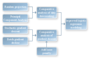
For the optimization of the logistic regression model, we primarily focus on optimizing from the row and column dimensions of the dataset. In selecting the methods, we employ a combination of stochastic projection and stochastic gradient descent to achieve optimization. However, the features resulting from stochastic projection dimensionality reduction still have room for further optimization, as there are a small number of redundant variables. Therefore, we add Lasso on the basis of stochastic gradient descent for further feature screening, aiming to improve the accuracy of the model.
Traditional dimensionality reduction methods, such as PCA and SVD, can indeed realize data dimensionality reduction. However, their disadvantage lies in the fact that the dimensionality reduction process itself requires a significant amount of computational time and resources, which is almost equivalent to the computing cost incurred before dimensionality reduction. Additionally, in the process of updating model parameters, ordinary gradient descent exhibits slow convergence when dealing with large sample sets, resulting in high computational demands, time complexity, and space complexity. This makes such methods less suitable for large-scale datasets. Therefore, this paper primarily focuses on investigating the impact of data dimensionality reduction and gradient descent on the classification effectiveness of machine learning.
In common optimization algorithms, we usually use gradient descent including batch gradient descent and stochastic gradient descent.
In terms of training speed, stochastic gradient descent iterates with only one sample at a time, resulting in a very fast training speed. On the contrary, batch gradient descent is significantly slower when dealing with a large sample size. However, in terms of accuracy, stochastic gradient descent uses only one sample to determine the direction of the gradient, leading to a parameter solution that may not be optimal. Nevertheless, it can still achieve good accuracy results. Additionally, from the perspective of utilizing sample information effectively, stochastic gradient descent and non-stochastic algorithms can be more efficient, especially when the information is redundant. Stochastic gradient descent selects one sample for updating each time, and it is possible to achieve convergence by using all the samples, thereby making full use of the effective information contained in the sample.
In terms of convergence of the algorithm, the batch gradient descent converges linearly in the strongly convex case, and in the worst case, it needs to converge at least \(O\left(\log \left(\frac{1}{\varepsilon } \right)\right)\) time to achieve the accuracy of Eq. (13): \[\label{GrindEQ__13_} \left\| \sum _{i=1}^{n}f_{i} \left(x_{t} \right)-f^{*} \right\| \le \varepsilon . \tag{13}\] Since batch gradient descent needs to compute \(n\) sample at a time, the total computational complexity of batch gradient descent is \(O\left(\log \left(\frac{1}{\varepsilon } \right)\right)^{*} O\left(\log \left(\frac{1}{\varepsilon } \right)\right)\).
For stochastic gradient descent, to achieve the accuracy of Eq. (14): \[\label{GrindEQ__14_} E\left[\left\| \sum _{i=1}^{n}f_{i} \left(x_{t} \right)-f^{*} \right\| \right]\le \varepsilon . \tag{14}\]
In the classification model of this paper, the logistic regression model is solved using stochastic gradient descent to solve the logistic regression, and in the process of partial derivation of the loss function, the stochastic gradient descent of logistic regression can be obtained in the form of: \[\label{GrindEQ__15_} \theta _{j+1} =\theta _{j} -\alpha \left(h_{\theta } \left(x^{i} \right)-y^{i} \right)x^{i} . \tag{15}\]
Proximal gradient descent is an important method for solving nonsmooth problems and one of the solution methods for solving Lasso’s problem, consider such a function problem: \[\label{GrindEQ__16_} {\mathop{\min }\limits_{x\in R^{d} }} f(x)=g(x)+h(x) , \tag{16}\] where \(g(x)\) and \(h(x)\) are both convex functions, but \(g(x)\) is smooth and \(h(x)\) is non-smooth. The most typical example of this type of problem is the least squares method based on the L1 paradigm, with the problem being: \[\label{GrindEQ__17_} {\mathop{\min }\limits_{x\in R^{d} }} \frac{1}{2} \left\| Ax-b\right\| ^{2} +\lambda \left\| x\right\| _{1} . \tag{17}\] The proximal gradient method requires the computation of neighboring operators at each iteration, see Eq. (18): \[\label{GrindEQ__18_} y={\mathop{\arg \min }\limits_{x\in R^{d} }} \frac{L}{2} \left\| x-y\right\| ^{2} +h(x) , \tag{18}\] where \(L\) is the Lipschitz constant for a \(g\)-gradient, i.e., there exists a constant \(L>0\) such that: \[\label{GrindEQ__19_} \left\| g{'} (x)-g{'} (x)\right\| \le L\left\| x{'} -x\right\| . \tag{19}\] This is a standard assumption for differentiable optimization, and if \(g\) is second-order differentiable, we base our Taylor expansion around \(x\): \[\label{GrindEQ__20_} g(y)\simeq g(x)+\left\langle g{'} (x),y-x\right\rangle +\frac{\mu }{2} \left\| y-x\right\| ^{2} . \tag{20}\] Rearranging the above equations gives: \[\label{GrindEQ__21_} g(y)\simeq \frac{L}{2} \left\| x-\left(x_{k} -\frac{1}{L} \nabla g\left(x_{k} \right)\right)\right\| _{2}^{2} +\varphi (x_{k} ) , \tag{21}\] where \(\varphi \left(x_{k} \right)\) is a constant that can be neglected. It follows from equation (21) that the minimum value of \(g(x)\) is obtained in equation (22): \[\label{GrindEQ__22_} x_{k+1} =x_{k} -\frac{1}{L} \nabla g\left(x_{k} \right) . \tag{22}\] When the non-smooth penalty term L1 is added, the minimax idea above is analogized to the case where the penalty term is added: \[\label{GrindEQ__23_} x_{k+1} ={\mathop{\arg \min }\limits_{x\in R^{d} }} \frac{L}{2} \left\| x-\left(x_{k} -\frac{1}{L} \nabla g\left(x_{k} \right)\right)\right\| _{2}^{2} +\lambda \left\| x\right\| _{1} . \tag{23}\] Proximal gradient descent to solve Lasso’s problem can be understood as one can first compute Eq. (22), treating \(x_{k+1}\) as \(z\), and then solve Eq. (24): \[\label{GrindEQ__24_} {\mathop{\arg \min }\limits_{x\in R^{d} }} \frac{L}{2} \left\| x-z\right\| _{2}^{2} +\lambda \left\| x\right\| _{1} . \tag{24}\] To achieve a screening variable. In a theoretical sense, soft thresholding generally solves the following problem: \[\label{GrindEQ__25_} {\mathop{\arg \min }\limits_{x\in R^{d} }} \left\| X-B\right\| _{2}^{2} +\lambda \left\| X\right\| _{1}. \tag{25}\] From a paradigm point of view, we can split this equation into: \[\label{GrindEQ__26_} \begin{array}{rcl} {F(X)} & {=} & {\left\| X-B\right\| _{2}^{2} +\lambda \left\| X\right\| _{1} }. \end{array} \tag{26}\] After splitting Eq. can be transformed into solving a small problem and there is no interaction between different \(x\)’s, see Eq. (27): \[\label{GrindEQ__27_} f(x)=(x-b)^{2} +\lambda |x| . \tag{27}\] The derivative of the function can be obtained: \[\label{GrindEQ__28_} \frac{df(x)}{dx} =2(x-b)+\lambda sgn(x), \tag{28}\] where \(sgn(x)\) is the sign function and we assume that the partial derivative is zero. \[\label{GrindEQ__29_} x=b-\frac{\lambda }{2} sgn(x) . \tag{29}\] For \(b\), there exist three different cases of solutions, and the minimum value of the function takes values in this state, see equation (30): \[\label{GrindEQ__30_} \arg \min f(x)=\left\{\begin{array}{ll} {b+\lambda /2,} & {{\rm b}<-\lambda /2}, \\ {0,} & {|b|\le \lambda /2}, \\ {b-\lambda /2,} & {{\rm b}>\lambda /2}. \end{array}\right. \tag{30}\] We can see that \(f(x)\) and \(F(x)\) are only different for variable \(b\) and independent variable \(x\). The function expressions are still approximately the same, so \(F(x)\) can also be expressed in terms of the above solution. Its closed-form solution can be found as Eq. (31): \[\label{GrindEQ__31_} x_{k+1}^i = \begin{cases} z^i – \frac{\lambda}{L}, & \frac{\lambda}{L}< z^i, \\ 0, & \left|z^i\right| \leq \frac{\lambda}{L}, \\ z^i + \frac{\lambda}{L}, & \frac{\lambda}{L}> z^i, \end{cases} \tag{31}\] Where \(x_{k+1} {}^{i}\) and \(z^{i}\) are the \(i\)th each component of \(x_{k+1}\) and \(z\) respectively. So from the above we can get that by proximal gradient descent we can minimize the Lasso and other Lasso based paradigms to reach the solution quickly.
The Lasso-logistic regression model is solved by a combination of stochastic gradient descent and proximal gradient descent methods. In this case, the problem to be solved by proximal gradient descent is Eq. (32): \[\label{GrindEQ__32_} {\mathop{\min }\limits_{{\rm x}\in R^{d} }} f(x)=g(x)+h(x) ,\tag{32}\] where \(g(x)\) is a smooth convex function and \(h(x)\) is a relatively simple convex function, but not trivial. In machine learning, we also often encounter optimization problems of this form, given a column of data \((a_{1} ,b_{1} ),\ldots ,(a_{n} ,b_{n} )\), hypothetically: \[\label{GrindEQ__33_} g_{i} (x)=\log \left(1+\exp \left(-b_{i} x^{T} a_{i} \right)\right),h(x)=\lambda \left\| x\right\| _{1} . \tag{33}\] This is a logistic regression optimization problem with the addition of a regular term, and in order to solve this problem, our conventional approach is to use proximal gradient descent, which can be described as Eq. (34): \[\label{GrindEQ__34_} x_{k+1} =prox_{\eta _{k} h} \left(x_{k} -\eta _{k} \nabla g\left(x_{k} \right)\right), \tag{34}\] where \(prox\) is the approximation operator, and the solution of the approximation operator generally needs to be transformed into Eq. (35): \[\label{GrindEQ__35_} prox_{\eta h} (y)={\mathop{\arg \min }\limits_{x\in R^{a} }} \left\{\frac{1}{2} \left\| x-y\right\| ^{2} +\eta \left\| x\right\| _{1} \right\} . \tag{35}\] The stochastic transformation of proximal gradient descent is stochastic proximal gradient descent (SPGD), in which at each iteration \(k=1,2,\ldots\), we randomly select \(i_{k}\) from \(\{ 1,2,\ldots ,n\}\) to update the parameters in the form of Eq. (36): \[\label{GrindEQ__36_} x_{k+1} =prox_{\eta _{k} h} \left(x_{k} -\eta _{k} \nabla g_{i_{k} } \left(x_{k} \right)\right) . \tag{36}\] Stochastic proximal gradient descent has the same structure as proximal gradient descent, but the advantage over proximal gradient descent is that at each iteration, stochastic forced gradient descent only needs to compute a single gradient \(\nabla g_{i_{k} } \left(x_{k} \right)\), in contrast to proximal gradient descent, which uses all of the samples \(N\) each time, and thus the computational cost of stochastic proximal gradient descent is \(1/N\) of the cost of proximal gradient descent.
This paper focuses on analyzing the data of Brent crude oil from May to June 2024.80% of the crude oil price data is used as a training set and the rest of the data is used as a test set to predict the upward and downward trend of Brent oil price. The opening price, high price, low price, closing price, and volume of Brent crude oil from May to June were obtained through Wind Financial Terminal.
It is generally accepted that long-term forecasting models should incorporate fundamental indicators, while short-term forecasting models, such as daily forecasting models, should primarily focus on technical indicators due to the lagging nature of fundamental data. This paper focuses on predicting the short-term upward and downward trends of crude oil prices. We selected 19 technical indicators as predictor variables and the rise and fall of the closing price as response variables. Five logistic regression models, namely traditional logistic regression, Ridge, Lasso, Elastic Net, and MCP, are utilized for comparison with the model proposed in this paper to predict the upward and downward trends of crude oil prices. The 19 indicators are WMA, DEMA, ADX, MACD, CCI, Mo, RSI, ATR, CLV, CMF, CMO, EMV, MFI, ROC, VHF, SAR, TRIX, WPR, and SNR.
In the following section, we utilize the test set and ROC surface analysis method to compare the prediction accuracy of the five logistic regression models with the model proposed in this paper. To visualize the comparison between the prediction results of these five models and the prediction results of the improved logistic regression model presented in this paper, we tabulate the prediction results of the logistic regression model with the technical indicators. Table 1 displays the prediction classes based on the prediction classes obtained from the training set and the actual classes provided by the test set, allowing us to establish a two-class confusion matrix.
The traditional logistic regression model predicts that the crude oil price will rise a total of 298 times, with actual rises occurring 202 times and actual falls occurring 96 times. It predicts that the international oil price will fall 248 times, with actual falls occurring 186 times and actual rises occurring 62 times. In contrast, the improved logistic regression algorithm proposed in this paper predicts a rise a total of 303 times, with actual rises occurring up to 227 times and prediction errors occurring 76 times. It predicts a fall 258 times, with correct predictions occurring 199 times and prediction errors occurring 59 times. The model proposed in this paper is significantly better than the traditional logistic regression model, and also outperforms other penalized logistic regression models.
| Logistic | 1(Observed rise) | 2(Observation fall) | Ridge | 1(Observed rise) | 2(Observation fall) |
| 1(Forecast to rise) | 202 | 96 | 1(Forecast to rise) | 168 | 68 |
| 2(Forecast to fall) | 62 | 186 | 2(Forecast to fall) | 106 | 194 |
| Lasso | 1(Observed rise) | 2(Observation fall) | Elastic Net | 1(Observed rise) | 2(Observation fall) |
| 1(Forecast to rise) | 180 | 79 | 1(Forecast to rise) | 199 | 88 |
| 2(Forecast to fall) | 93 | 182 | 2(Forecast to fall) | 74 | 173 |
| MCP | 1(Observed rise) | 2(Observation fall) | This algorithm | 1(Observed rise) | 2(Observation fall) |
| 1(Forecast to rise) | 207 | 88 | 1(Forecast to rise) | 227 | 76 |
| 2(Forecast to fall) | 66 | 173 | 2(Forecast to fall) | 59 | 199 |
Then their sensitivity, specificity, and overall accuracy were analyzed.
Table 2 shows the results of analyzing the sensitivity, specificity, and overall accuracy of the six models. It can be seen that the overall accuracy rate of traditional logistic regression model is 0.726, while the overall accuracy rate of this paper’s algorithm is 0.767, which is obviously better than that of traditional logistic regression.The accuracy rates of Ridge, Lasso, and Elastic Net are lower than that of traditional logistic regression, which are 0.696, 0.696, and 0.716, respectively, which means that the prediction accuracy is not necessarily improved just because a penalty term is added to the original function. will be improved.
| Evaluation criteria | Logistic | Ridge | Lasso | Elastic Net | MCP | This algorithm |
| Sensitivity | 0.791 | 0.624 | 0.675 | 0.751 | 0.783 | 0.783 |
| Specificity | 0.663 | 0.764 | 0.717 | 0.68 | 0.68 | 0.749 |
| Overall accuracy | 0.726 | 0.696 | 0.696 | 0.716 | 0.733 | 0.767 |
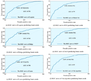
Because the overall accuracy is the simplest index to evaluate the prediction, but it cannot fully reflect the loss corresponding to the two types of errors. Therefore, the ROC curve is introduced to evaluate the accuracy of prediction, which mainly utilizes different thresholds to calculate the sensitivity and specificity, and draws the ROC curve for evaluating the prediction accuracy.The area AUC under the ROC curve evaluates the classification effect of the classifier: the larger the AUC is, the better the classification effect is. When AUC = 1, the classifier is nearly perfect, and accurate prediction classes can be obtained no matter what threshold is set when using this classifier prediction model. When 0.5 \(\mathrm{<}\) AUC \(\mathrm{<}\) 1, the classifier is better than random guessing. When AUC=0.5, the classifier performs as bad as random guessing. When AUC \(\mathrm{<}\) 0.5, the classifier performs worse than random guessing.
Figure 2 shows the ROC curves of the six models predicting the rise and fall of the international Brent crude oil price. From the figure, it can be seen that the AUCs of the traditional logistic regression model, Ridge model, Lasso model, EN model, MCP model and this paper’s model are 0.753, 0.63, 0.758, 0.779, 0.781, and 0.787, respectively.The AUC of this paper’s improved logistic regression model is higher than that of the traditional logistic regression model by 0.034, which is also significantly higher than that of the other penalized logistic regression models. Combined with the overall accuracy in Table 2, it can be concluded that the improved logistic regression model of this paper with technical indicators performs better than the traditional logistic regression, ridge regression, Lasso and elastic net prediction with technical indicators, and performs better in predicting the upward and downward trend of the crude oil price, and the effectiveness of the improved algorithm of the logistic regression of this paper is verified.
In this paper, the improved logistic regression model is used to make short-term predictions of crude oil prices for different types of emergencies, and the different price ranges and probabilities of crude oil prices that may occur in the next 24 hours are given.
Table 3 shows the results of crude oil price forecasts in the event of a natural disaster. As can be seen from Table 3, when natural disasters occur, the probability that international crude oil prices will fluctuate between 0\(\mathrm{\sim}\)4 US dollars in the next 24 hours is the largest, with an average probability of 0.58666. The second is a fluctuation of 4\(\mathrm{\sim}\)10 US dollars, with an average probability of 0.39321. The probability of a fluctuation of more than $15 is the smallest, with an average probability of 0.05117.
Table 4 shows the results of crude oil price forecasts when important data exceeds expectations. As can be seen from Table 4, when economic data, monetary data, crude oil production and sales, inventories and other indicators are extremely inconsistent with expectations, the probability of international crude oil prices fluctuating between 4\(\mathrm{\sim}\)10 US dollars in the next 24 hours is the largest, with an average probability of 0.55345. The second is the fluctuation of 0\(\mathrm{\sim}\)4 US dollars, with an average probability of 0.37628. The probability of a fluctuation of more than $15 is the smallest, with an average probability of 0.04906.
| Time | P1:(0,4) | P2:(4,10) | P3:(10,15) | P4:(15,+$$\mathrm{\infty}$$) |
| 4:00 | 0.41749 | 0.51214 | 0.07294 | 0.04814 |
| 8:00 | 0.36751 | 0.55111 | 0.07733 | 0.05477 |
| 12:00 | 0.35649 | 0.57814 | 0.06448 | 0.05161 |
| 16:00 | 0.38393 | 0.53958 | 0.07192 | 0.05539 |
| 20:00 | 0.38352 | 0.53958 | 0.07763 | 0.05018 |
| 24:00 | 0.34864 | 0.59986 | 0.06805 | 0.03427 |
| Average | 0.37628 | 0.55345 | 0.07202 | 0.04906 |
This paper USES improved logical regression algorithm to predict international crude oil market, and compares the predictive energy of five other logical regression models, and draws the following conclusions:
After the training of the data set, the traditional logistic regression model predicts that the crude oil price will rise for a total of 298 times, and actually rises for 202 times and falls for 96 times. The improved logistic regression algorithm in this paper predicts rise a total of 303 times, the actual rise up to 227 times, the prediction error 76 times. The algorithm in this paper clearly provides more trading opportunities and a higher prediction success rate.
The overall accuracy of traditional logistic regression model is 0.726, while the overall accuracy of this paper’s algorithm is 0.767, which is obviously better than traditional logistic regression.The accuracy of Ridge, Lasso, and Elastic Net is lower than that of traditional logistic regression, which is 0.696, 0.696, and 0.716, respectively, which means that it is clear that not by adding a penalty term to the original function the prediction accuracy is bound to be improve.
The AUCs of the traditional logistic regression model, Ridge model, Lasso model, EN model, MCP model and this paper’s model are 0.753, 0.63, 0.758, 0.779, 0.781, 0.787, respectively, whereas this paper’s model is higher than the traditional logistic regression model by 0.034, which is significantly higher than other penalized logistic regression models. This paper’s model performs better in predicting the rising and falling trend of crude oil prices, and the effectiveness of the improved algorithm is verified.
When natural disaster-type emergencies occur, the probability that the international crude oil price will keep fluctuating between 0 and 4 U.S. dollars in the next 24 hours is the greatest, with an average probability of 0.58666. And when economic data, monetary data, crude oil production and sales, and stockpiles and other indexes are extremely out of line with the expectations, the probability that the international crude oil price will keep fluctuating between 4 and 10 U.S. dollars in the next 24 hours is the greatest, with an average probability of 0.55345.